Map Coloring: Hybrid DQM Sampler#

This example solves the same map coloring problem of Large Map Coloring to demonstrate Leap‘s hybrid discrete quadratic model (DQM) solver, which enables you to solve problems of arbitrary structure and size for variables with discrete values.

See Large Map Coloring for a description of the map coloring constraint satisfaction problem (CSP).

The Map Coloring advanced example demonstrates lower-level coding of a similar problem, which gives the user more control over the solution procedure but requires the knowledge of some system parameters (e.g., knowing the maximum number of supported variables for the problem). Example Problem With Many Variables demonstrates the hybrid approach to problem solving in more detail by explicitly configuring the classical and quantum workflows.

Example Requirements#

The code in this example requires that your development environment have Ocean software and be configured to access SAPI, as described in the Initial Set Up section.

Note

This example requires a minimal understanding of the penalty model approach to solving problems by minimizing penalties. In short, you formulate the problem using positive values to penalize undesirable outcomes; that is, the problem is formulated as an objective function where desirable solutions are those with the lowest values. This is demonstrated in Leap‘s Structural Imbalance demo, introduced in the Boolean AND Gate example, and comprehensively explained in the Problem Solving Handbook.

Solution Steps#

Section Workflow Steps: Formulation and Sampling describes the problem-solving workflow as consisting of two main steps: (1) Formulate the problem as an objective function in a supported model and (2) Solve your model with a D-Wave solver.

In this example, a DQM is created to formulate the problem and submitted to the Leap hybrid DQM solver, hybrid_binary_quadratic_model_version<x>.

Formulate the Problem#

This example uses the NetworkX read_adjlist() function to read a text file, usa.adj, containing the states of the USA and their adjacencies (states with a shared border) into a graph. The original map information was found on write-only blog of Gregg Lind and looks like this:

# Author Gregg Lind
# License:  Public Domain.    I would love to hear about any projects you use if it for though!
#
AK,HI
AL,MS,TN,GA,FL
AR,MO,TN,MS,LA,TX,OK
AZ,CA,NV,UT,CO,NM
CA,OR,NV,AZ
CO,WY,NE,KS,OK,NM,AZ,UT

# Snipped here for brevity

You can see in the first non-comment line that the state of Alaska (“AK”) has Hawaii (“HI”) as an adjacency and that Alabama (“AL”) shares borders with four states.

>>> import networkx as nx
>>> G = nx.read_adjlist('usa.adj', delimiter = ',')   

Graph G now represents states as vertices and each state’s neighbors as shared edges.

>>> states = G.nodes        
>>> borders = G.edges       

You can now create a dimod.DiscreteQuadraticModel object to represent the problem. Because any planar map can be colored with four colors or fewer, represent each state with a discrete variable that has four cases (binary variables can have two values; discrete variables can have some arbitrary number of cases).

For every pair of states that share a border, set a quadratic bias of \(1\) between the variables’ identical cases and \(0\) between all different cases (by default, the quadratic bias is zero). Such as penalty model adds a value of \(1\) to solutions of the DQM for every pair of neighboring states with the same color. Optimal solutions are those with the fewest such neighboring states.

>>> import dimod
...
>>> colors = [0, 1, 2, 3]
...
>>> dqm = dimod.DiscreteQuadraticModel()
>>> for state in states:            
...    dqm.add_variable(4, label=state)
>>> for state0, state1 in borders:          
...    dqm.set_quadratic(state0, state1, {(color, color): 1 for color in colors})

Solve the Problem by Sampling#

D-Wave’s quantum cloud service provides cloud-based hybrid solvers you can submit arbitrary BQMs and DQMs to. These solvers, which implement state-of-the-art classical algorithms together with intelligent allocation of the quantum processing unit (QPU) to parts of the problem where it benefits most, are designed to accommodate even very large problems. Leap’s solvers can relieve you of the burden of any current and future development and optimization of hybrid algorithms that best solve your problem.

Ocean software’s dwave-system LeapHybridDQMSampler class enables you to easily incorporate Leap’s hybrid DQM solvers into your application. The solution printed below is truncated.

>>> from dwave.system import LeapHybridDQMSampler
...
>>> sampleset = LeapHybridDQMSampler().sample_dqm(dqm,
...                 label='SDK Examples - Map Coloring DQM')  
...
>>> print("Energy: {}\nSolution: {}".format(
...        sampleset.first.energy, sampleset.first.sample))  
Energy: 0.0
Solution: {'AK': 0, 'AL': 0, 'MS': 3, 'TN': 1, 'GA': 2, 'FL': 3, 'AR': 2,
# Snipped here for brevity

The energy value of zero above signifies that this first (best) solution found has accumulated no penalties, meaning no pairs of neighboring states with the same color.

Note

The next code requires Matplotlib.

Plot the best solution.

>>> import matplotlib.pyplot as plt       
>>> node_list = [list(G.nodes)[x:x+10] for x in range(0, 50, 10)]   
>>> node_list[4].append('ND')     
# Adjust the next line if using a different map
>>> nx.draw(G, pos=nx.shell_layout(G, nlist = node_list), with_labels=True,
...         node_color=list(sampleset.first.sample.values()), node_size=400,
...         cmap=plt.cm.rainbow)                 
>>> plt.show()    

The graphic below shows the result of one such run.

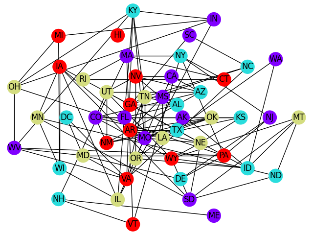
One solution `hybrid_binary_quadratic_model_version1` found for the USA map-coloring problem.#