Sampling: Minimizing the Objective#

Having formulated an objective function that represents your problem as described in the Formulation: Objectives and Models section, you sample this quadratic model (QM) or nonlinear model for solutions. Ocean software provides quantum, classical, and quantum-classical hybrid samplers that run either remotely (for example, in D-Wave’s Leap environment) or locally on your CPU. These compute resources are known as solvers.

Note

Some classical samplers actually brute-force solve small problems rather than sample, and these are also referred to as “solvers”.

Ocean’s samplers enable you to submit your problem to remote or local compute resources (solvers) of different types:

Hybrid Solvers such as Leap’s hybrid_binary_quadratic_model_version<x> solver or hybrid_nonlinear_program_version<x>.
Classical Solvers such as ExactSolver for exact solutions to small problems
Quantum Solvers such as the Advantage system.

Submit the Model to a Solver#

The example code below submits a BQM representing a Boolean AND gate (see also the Example: BQM for a Boolean Circuit section) to a Leap hybrid solver. In this case, dwave-system’s LeapHybridSampler is the Ocean sampler and the remote compute resource selected might be Leap hybrid solver hybrid_binary_quadratic_model_version<x>.

>>> from dimod.generators import and_gate
>>> from dwave.system import LeapHybridSampler
>>> bqm = and_gate('x1', 'x2', 'y1')
>>> sampler = LeapHybridSampler()    
>>> answer = sampler.sample(bqm)   
>>> print(answer)    
  x1 x2 y1 energy num_oc.
0  1  1  1    0.0       1
['BINARY', 1 rows, 1 samples, 3 variables]

Improve the Solutions#

For complex problems, you can often improve solutions and performance by applying some of Ocean software’s preprocessing, postprocessing, and diagnostic tools.

Additionally, when submitting problems directly to a D-Wave system (Quantum Solvers), you can benefit from some advanced features (for example features such as spin-reversal transforms and anneal offsets, which reduce the impact of possible analog and systematic errors) and the techniques described in the Problem Solving Handbook guide.

Example: Preprocessing#

dwave-preprocessing provides algorithms such as roof duality, which fixes some of a problem’s variables before submitting to a sampler.

As an illustrative example, consider the binary quadratic model, \(x + yz\). Clearly \(x=0\) for all the best solutions (variable assignments that minimize the value of the model) because any assignment of variables that sets \(x=1\) adds a value of 1 compared to assignments that set \(x=0\). (On the other hand, assignment \(y=0, z=0\), assignment \(y=0, z=1\), and assignment \(y=1, z=0\) are all equally good.) Therefore, you can fix variable \(x\) and solve a smaller problem.

>>> from dimod import BinaryQuadraticModel
>>> from dwave.preprocessing import roof_duality
>>> bqm = BinaryQuadraticModel({'x': 1}, {('y', 'z'): 1}, 0,'BINARY')
>>> roof_duality(bqm)
(0.0, {'x': 0})

For problems with hundreds or thousands of variables, such preprocessing can significantly improve performance.

Example: Diagnostics#

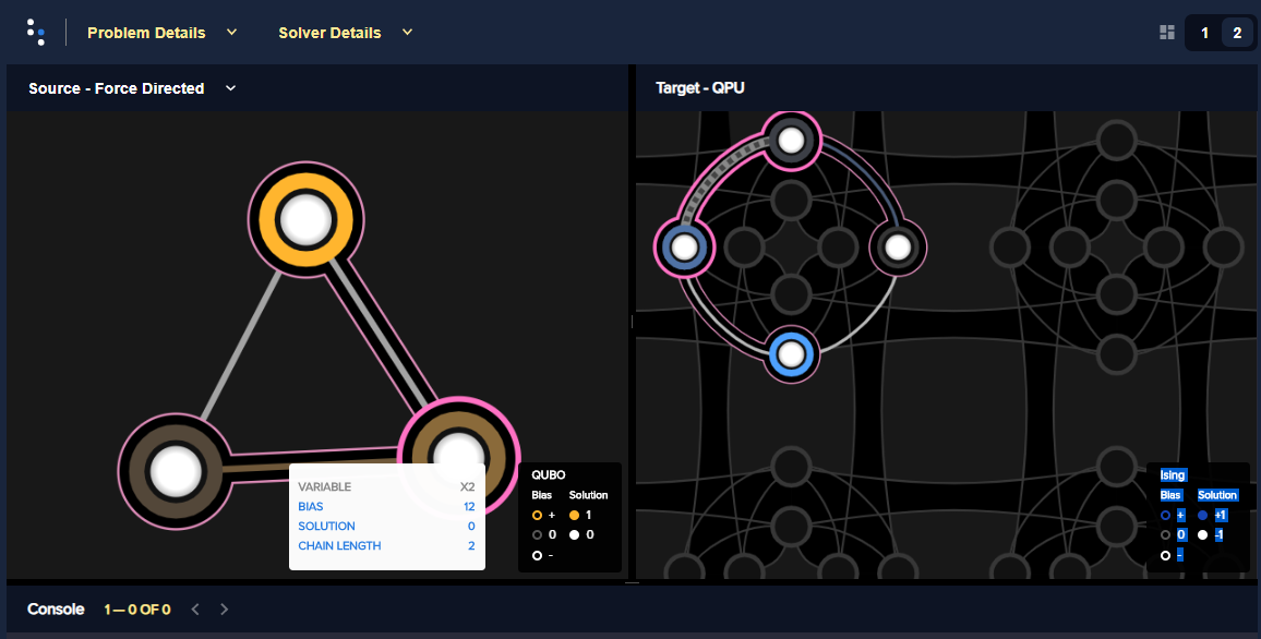
When sampling directly on the D-Wave QPU, the mapping from problem variables to qubits, minor-embedding, can significantly affect performance. Ocean tools perform this mapping heuristically so simply rerunning a problem might improve results. Advanced users may customize the mapping by directly using the minorminer tool, setting a minor-embedding themselves, or using D-Wave’s problem-inspector tool.

For example, the Boolean AND Gate example submits the BQM representing an AND gate to a D-Wave system, which requires mapping the problem’s logical variables to qubits on the QPU. The code below invokes D-Wave’s problem-inspector tool to visualize the minor-embedding.

>>> import dwave.inspector
>>> dwave.inspector.show(response)   

View rendered by Ocean's problem inspector. — View of the logical and embedded problem rendered by Ocean’s problem inspector. The AND gate’s original BQM is represented on the left; its embedded representation on a D-Wave system, on the right, shows a two-qubit chain (qubits 176 and 180) for variable \(x2\). The tool is helpful in visualizing the quality of your embedding.#

Example: Postprocessing#

Example Postprocessing with a Greedy Solver improves samples returned from a QPU by post-processing with a classical greedy algorthim.