Postprocessing with a Greedy Solver#

This example uses explicit postprocessing to improve results returned from a quantum computer.

Typically, Ocean tools do some minimal, implicit postprocessing; for example, when you use embedding tools to map problem variables to qubits, broken chains (differing states of the qubits representing a variable) may be resolved by majority vote: Ocean sets the variable’s value based on the state returned from the majority of the qubits in the chain. You can often improve results, at a low cost of classical processing time, by postprocessing.

dwave-greedy provides an implementation of a steepest-descent solver, SteepestDescentSolver, for binary quadratic models. This example runs this classical algorithm initialized from QPU samples to find minima in the samples’ neighbourhoods.

The purpose of this example is to illustrate the benefit of postprocessing results from non-deterministic samplers such as quantum computers.

Example Requirements#

The code in this example requires that your development environment have Ocean software and be configured to access SAPI, as described in the Initial Set Up section.

Solution Steps#

Section Workflow Steps: Formulation and Sampling describes the problem-solving workflow as consisting of two main steps: (1) Formulate the problem as an objective function in a supported form of quadratic model (QM) and (2) Solve your QM with a D-Wave solver.

This example adds an optional step of postprocessing the returned solution.

Formulate the Problem#

This example uses a synthetic problem for illustrative purposes: for all couplers of a QPU, it sets quadratic biases equal to random integers between -5 to +5.

# Create a native Ising problem
from dwave.system import DWaveSampler
import numpy as np

sampler = DWaveSampler()
h = {v: 0.0 for v in sampler.nodelist}
J = {tuple(c): np.random.choice(list(range(-5, 6))) for c in sampler.edgelist}

Solve the Problem and Run Postprocessing#

Because the problem sets values of the Ising problem based on the qubits and couplers of a selected QPU (a native problem), you can submit it directly to that QPU without embedding. The SampleSet returned from the QPU is used to initialize SteepestDescentSolver: for each sample, this classical solver runs its steepest-descent algorithm to find the closest minima.

from greedy import SteepestDescentSolver

solver_greedy = SteepestDescentSolver()

sampleset_qpu = sampler.sample_ising(h, J, \
                                     num_reads=100, \
                                     answer_mode='raw', \
                                     label='SDK Examples - Postprocessing')
# Postprocess
sampleset_pp = solver_greedy.sample_ising(h, J, initial_states=sampleset_qpu)

You can graphically compare the results before and after the postprocessing.

Note

The next code requires Matplotlib.

>>> import matplotlib.pyplot as plt    
...
>>> plt.plot(list(range(100)), sampleset_qpu.record.energy, 'b.-',
...                            sampleset_pp.record.energy, 'r^-') 
>>> plt.legend(['QPU samples', 'Postprocessed Samples'])          
>>> plt.xlabel("Sample")    
>>> plt.ylabel("Energy")    
>>> plt.show()              

The image below shows the result of one particular execution on an Advantage QPU.

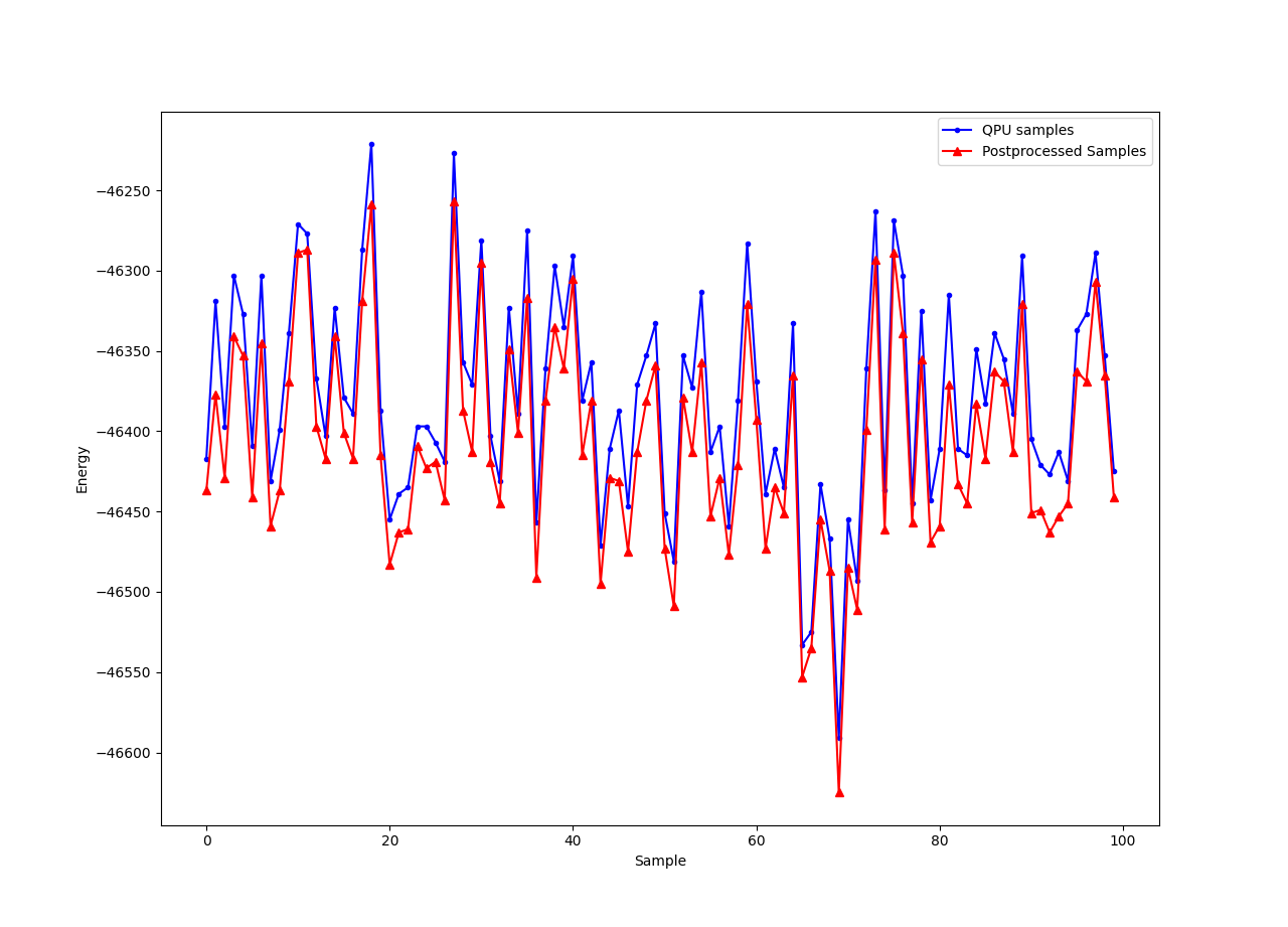
QPU samples before and after postprocessing with a steepest-descent solver.#

For reference, this execution had the following median energies before and after postprocessing, and for a running the classical solver directly on the problem, in which case it uses random samples to initiate its local searches.

sampleset_greedy = solver_greedy.sample_ising(h, J, num_reads=100)

>>> print("Energies: \n\t
...        SteepestDescentSolver: {}\n\t
...        QPU samples: {}\n\t
...        Postprocessed: {}".format(
...        np.median(sampleset_greedy.record.energy),
...        np.median(sampleset_qpu.record.energy),
...        np.median(sampleset_pp.record.energy)))       
Energies:
        SteepestDescentSolver: -39834.0
        QPU samples: -46387.0
        Postprocessed: -46415.0