Map Coloring#

This example solves a map-coloring problem. It demonstrates using a D-Wave quantum computer to solve a more complex constraint satisfaction problem (CSP) than that solved in the Constrained Scheduling example.

Constraint satisfaction problems require that all a problem’s variables be assigned values, out of a finite domain, that result in the satisfying of all constraints. The map-coloring CSP requires that you assign a color to each region of a map such that any two regions sharing a border have different colors.

Coloring a map of Canada with four colors.#

The constraints for the map-coloring problem can be expressed as follows:

Each region is assigned one color only, of \(C\) possible colors.
The color assigned to one region cannot be assigned to adjacent regions.

Example Requirements#

The code in this example requires that your development environment have Ocean software and be configured to access SAPI, as described in the Initial Set Up section.

Solution Steps#

Section Workflow Steps: Formulation and Sampling describes the problem-solving workflow as consisting of two main steps: (1) Formulate the problem as an objective function in a supported form of quadratic model (QM) and (2) Solve your QM with a D-Wave solver.

This example formulates the problem as a binary quadratic model (BQM) by using unary encoding to represent the \(C\) colors: each region is represented by \(C\) variables, one for each possible color, which is set to value \(1\) if selected, while the remaining \(C-1\) variables are \(0\). It then solves the BQM on a D-Wave quantum computer.

This example represents the problem’s constraints as penalties and creates an objective function by summing all penalty models.

Note

This problem can be expressed more simply using variables with multiple values; for example, provinces could be represented by discrete variables with values {yellow, green, blue, red} instead of four binary variables (one for each color). For such problems a discrete quadratic model (DQM) is a better choice.

In general, problems with constraints are more simply solved using a constrained quadratic model (CQM) and appropriate hybrid CQM solver, as demonstrated in the Bin Packing and Stock-Sales Strategy in a Simplified Market examples; however, the purpose of this example is to demonstrate solution directly on a D-Wave quantum computer.

The full workflow is as follows:

Formulate the problem as a graph, with provinces represented as nodes and shared borders as edges, using 4 binary variables (one per color) for each province.
Create one-hot penalties for each node to enforce the constraint that each province is assigned one color only.
Create penalties for each edge to enforce the constraint that no two neighbors have the same color.
Add all the constraints into a single BQM.
Sample the BQM.
Plot a feasible solution (a solution that meets all the constraints).

Formulate the Problem#

This example finds a solution to the map-coloring problem for a map of Canada using four colors (the sample code can easily be modified to change the number of colors or use different maps). Canada’s 13 provinces are denoted by postal codes:

Canadian Provinces’ Postal Codes#
Code	Province	Code	Province
AB	Alberta	BC	British Columbia
MB	Manitoba	NB	New Brunswick
NL	Newfoundland and Labrador	NS	Nova Scotia
NT	Northwest Territories	NU	Nunavut
ON	Ontario	PE	Prince Edward Island
QC	Quebec	SK	Saskatchewan
YT	Yukon

Note

You can skip directly to the complete code for the problem here: Map Coloring: Full Code.

The example uses dimod to set up penalties and create a binary quadratic model, dwave-system to set up a D-Wave quantum computer as the sampler, and NetworkX to plot results.

>>> import networkx as nx
>>> import matplotlib.pyplot as plt    
>>> from dimod.generators import combinations
>>> from dimod import BinaryQuadraticModel, ExactSolver
>>> from dwave.system import DWaveSampler, EmbeddingComposite

Start by formulating the problem as a graph of the map with provinces as nodes and shared borders between provinces as edges; e.g., ('AB', 'BC') is an edge representing the shared border between British Columbia and Alberta.

>>> provinces = ['AB', 'BC', 'MB', 'NB', 'NL', 'NS', 'NT', 'NU', 'ON', 'PE',
...              'QC', 'SK', 'YT']
>>> neighbors = [('AB', 'BC'), ('AB', 'NT'), ('AB', 'SK'), ('BC', 'NT'), ('BC', 'YT'),
...              ('MB', 'NU'), ('MB', 'ON'), ('MB', 'SK'), ('NB', 'NS'), ('NB', 'QC'),
...              ('NL', 'QC'), ('NT', 'NU'), ('NT', 'SK'), ('NT', 'YT'), ('ON', 'QC')]

You can set four arbitrary colors. The strings chosen here are recognized by the Matplotlib graphics library, which is used for plotting a solution in the last step, to represent colors yellow, green, red, and blue respectively.

>>> colors = ['y', 'g', 'r', 'b']

The next steps represent the binary constraint satisfaction problem with a BQM that models the two types of constraints using penalty models.

Constraint 1: One Color Per Region#

In the code below, bqm_one_color uses a one-hot penalty model to formulate the constraint that each node (province) select a single color.

Hint

The following illustrative example shows a one-hot constraint on two variables, represented by the penalty model, \(2ab - a - b\). You can easily verify that the ground states (solutions with lowest values, zero in this case) are for variable assignments where just one of the variables has the value 1.

>>> bqm_one_hot = combinations(['a', 'b'], 1)
>>> print(bqm_one_hot)
BinaryQuadraticModel({'a': -1.0, 'b': -1.0}, {('b', 'a'): 2.0}, 1.0, 'BINARY')
>>> print(ExactSolver().sample(bqm_one_hot))
   a  b energy num_oc.
1  1  0    0.0       1
3  0  1    0.0       1
0  0  0    1.0       1
2  1  1    1.0       1
['BINARY', 4 rows, 4 samples, 2 variables]

Set a one-hot constraint on the four binary variables representing the possible colors for each province.

>>> bqm_one_color = BinaryQuadraticModel('BINARY')
>>> for province in provinces:
...   variables = [province + "_" + c for c in colors]
...   bqm_one_color.update(combinations(variables, 1))

As in the illustrative example above, the binary variables created for each province set linear biases of -1 and quadratic biases of 2 that penalize states where more than a single color is selected.

>>> print([variable for variable in bqm_one_color.variables if provinces[0] in variable])
['AB_y', 'AB_g', 'AB_r', 'AB_b']
>>> print(bqm_one_color.linear['AB_y'], bqm_one_color.quadratic['AB_y', 'AB_g'])
-1.0 2.0

Constraint 2: Different Colors for Adjacent Regions#

In the code below, bqm_neighbors represents the constraint that two nodes (provinces) with a shared edge (border) not both select the same color.

Hint

The following illustrative example shows an AND constraint on two variables, represented by the penalty model, \(1 - ab\). You can easily verify that the ground states (solutions with lowest values, zero in this case) are for variable assignment \(a = b = 1\).

>>> bqm_and = BinaryQuadraticModel({}, {'ab': -1}, 1, 'BINARY')
>>> print(ExactSolver().sample(bqm_and))
   a  b energy num_oc.
2  1  1    0.0       1
0  0  0    1.0       1
1  1  0    1.0       1
3  0  1    1.0       1
['BINARY', 4 rows, 4 samples, 2 variables]

Switching the sign of the quadratic coefficient to \(+1\) (and dropping the offset) now penalizes variable assignment \(a = b = 1\).

>>> bqm_and_plus = BinaryQuadraticModel({}, {'ab': 1}, 0, 'BINARY')
>>> print(ExactSolver().sample(bqm_and_plus))
   a  b energy num_oc.
0  0  0    0.0       1
1  1  0    0.0       1
3  0  1    0.0       1
2  1  1    1.0       1
['BINARY', 4 rows, 4 samples, 2 variables]

The code below sets quadratic coefficients to \(+1\) for interactions between neighboring provinces’ variables representing the same color, for example AB_y and BC_y (yellow for Alberta and British Columbia).

>>> bqm_neighbors  = BinaryQuadraticModel('BINARY')
>>> for neighbor in neighbors:
...   v, u = neighbor
...   interactions = [(v + "_" + c, u + "_" + c) for c in colors]
...   for interaction in interactions:
...      bqm_neighbors.add_quadratic(interaction[0], interaction[1], 1)

Create a BQM for the Problem#

The previous sections created BQMs that represent the two types of constraints. For some problems, such constraints are supplementary to an objective that needs to be minimized, but in this problem, any solution that meets the constraints is a good solution. The BQM that represents the map coloring problem is therefore a simple sum of the BQMs representing the constraints.

>>> bqm = bqm_one_color + bqm_neighbors

Sample the BQM#

Set up a D-Wave quantum computer as the sampler and request 1000 samples.

Note

The code below sets a sampler without specifying SAPI parameters. Configure a default solver as described in Configuring Access to Leap’s Solvers to run the code as is, or see dwave-cloud-client to access a particular solver by setting explicit parameters in your code or environment variables.

>>> sampler = EmbeddingComposite(DWaveSampler())       
>>> sampleset = sampler.sample(bqm, num_reads=1000,
...                            label='SDK Examples - Map Coloring BQM') 
...
>>> best = sampleset.first     

Verify that the quantum computer found a feasible solution.

>>> if best.energy > 0:        
...     print("Failed to color map. Try sampling again.")

Plot a Feasible Solution#

Note

The next code requires Matplotlib.

The function below plots the map as a graph with nodes set to the selected color for each province.

def plot_map(sample):
    G = nx.Graph()
    G.add_nodes_from(provinces)
    G.add_edges_from(neighbors)
    # Create a {province: selected color} dict
    color_map = {}
    for province in provinces:
      for c in colors:
       if sample[province + '_' + c]:
           color_map[province] = c
    # Plot with the selected colors
    node_colors = [color_map.get(node) for node in G.nodes()]
    nx.draw_circular(G, with_labels=True, node_color=node_colors, node_size=3000, cmap=plt.cm.rainbow)
    plt.show()

>>> plot_map(best.sample)    

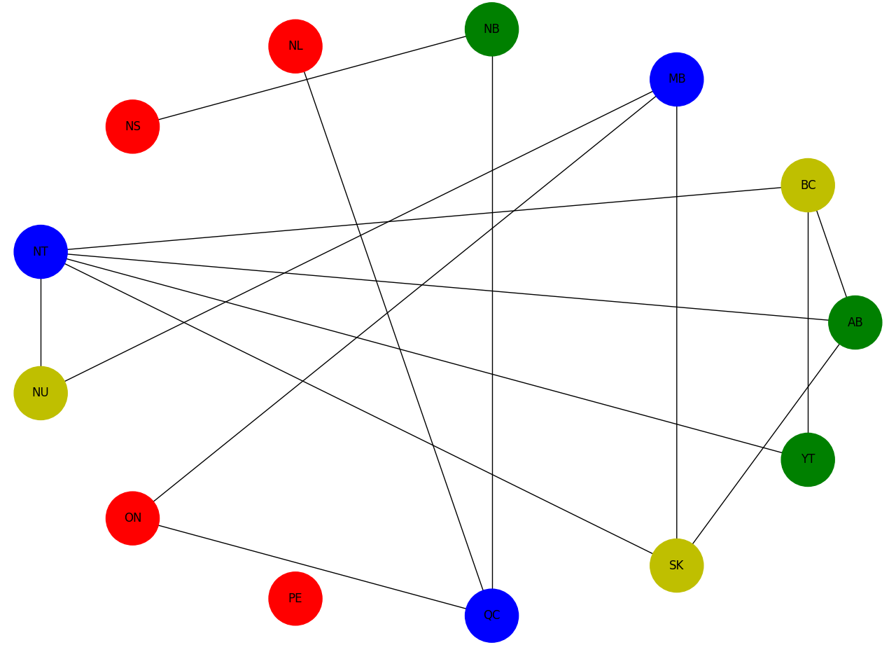
Solution for a map of Canada with four colors. The graph comprises 13 nodes representing provinces connected by edges representing shared borders. No two nodes connected by an edge share a color.#

Note

You can copy the complete code for the problem here: Map Coloring: Full Code.