Multiple-Gate Circuit#
This example solves a logic-circuit problem on a D-Wave quantum computer. It expands on the discussion in the Boolean AND Gate example about the effect of minor-embedding on performance, demonstrating different approaches to embedding.
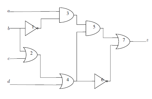
Circuit with 7 logic gates, 4 inputs (\(a, b, c, d\)), and 1 output (\(z\)). The circuit implements function \(z = \overline{b} (ac + ad + \overline{c}\overline{d})\).#
Example Requirements#
The code in this example requires that your development environment have Ocean software and be configured to access SAPI, as described in the Initial Set Up section.
For the optional graphics, you will also need the non-open-source problem-inspector Ocean package, which you may have chosen to install in the Install Contributor Ocean Tools section.
Formulating the Problem as a CSP#
Other examples (Boolean NOT Gate and Boolean AND Gate) show how a Boolean gate is represented as a constraint satisfaction problem (CSP) on a quantum computer. This example aggregates the resulting binary quadratic models (BQM) to do the same for multiple gates that constitute a circuit.
Small-Circuit Problem#
To start with, solve the circuit with 7 logic gates shown above.
The code below represents standard Boolean gates with BQMs provided by dimod BQM generators, represents the Boolean NOT operation by inverting the coefficients of the relevant variables, and sums the gate-level BQMs. The resulting aggregate BQM has its lowest value for variable assignments that satisfy all the constraints representing the circuit’s Boolean gates.
>>> from dimod.generators import and_gate, or_gate
...
>>> bqm_gate2 = or_gate('b', 'c', 'out2')
>>> bqm_gate3 = and_gate('a', 'b', 'out3')
>>> bqm_gate3.flip_variable('b')
>>> bqm_gate4 = or_gate('out2', 'd', 'out4')
>>> bqm_gate5 = and_gate('out3', 'out4', 'out5')
>>> bqm_gate7 = or_gate('out5', 'out4', 'z')
>>> bqm_gate7.flip_variable('out4')
...
>>> bqm = bqm_gate2 + bqm_gate3 + bqm_gate4 + bqm_gate5 + bqm_gate7
>>> print(bqm.num_variables)
9
This circuit is small enough to solve with a brute-force algorithm such as that
used by the ExactSolver class. Solve and
print all feasible solutions.
>>> from dimod import ExactSolver, drop_variables
...
>>> solutions = ExactSolver().sample(bqm).lowest()
>>> out_fields = [key for key in list(next(solutions.data(['sample'])))[0].keys() if 'out' in key]
>>> print(drop_variables(solutions, out_fields))
    a  b  c  d  z energy num_oc.
0   0  0  0  1  0    0.0       1
1   0  0  1  1  0    0.0       1
2   0  1  1  1  0    0.0       1
3   0  1  0  1  0    0.0       1
4   1  1  0  1  0    0.0       1
5   1  1  1  1  0    0.0       1
6   1  1  1  0  0    0.0       1
7   1  1  0  0  0    0.0       1
8   0  1  0  0  0    0.0       1
9   0  1  1  0  0    0.0       1
10  0  0  1  0  0    0.0       1
11  1  0  0  1  1    0.0       1
12  1  0  1  1  1    0.0       1
13  1  0  1  0  1    0.0       1
14  1  0  0  0  1    0.0       1
15  0  0  0  0  1    0.0       1
['BINARY', 16 rows, 16 samples, 5 variables]
Brute-force algorithms are not effective for large problems.
Large-Circuit Problem#
In the figure below, the 7-gates circuit solved above is replicated with the outputs connected through a series of XOR gates.
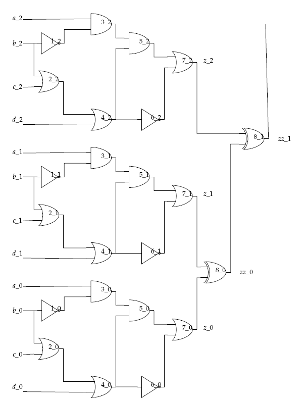
Multiple replications of the 7-gates circuit (\(z = \overline{b} (ac + ad + \overline{c}\overline{d})\)) connected by XOR gates.#
The circuit_bqm function defined below replicates, for a specified number
of circuits, the BQM developed above and connects the outputs through a cascade
of XOR gates.
>>> from dimod import BinaryQuadraticModel, quicksum
>>> from dimod.generators import and_gate, or_gate, xor_gate
...
>>> def circuit_bqm(n: int = 3) -> BinaryQuadraticModel:
...       "Create a BQM for n replications of the 7-gate circuit."
...
...       if n < 2:
...          raise ValueError("n must be at least 2")
...
...       bqm_gate2 = [or_gate(f"b_{c}", f"c_{c}", f"out2_{c}") for c in range(n)]
...       bqm_gate3 = [and_gate(f"a_{c}", f"b_{c}", f"out3_{c}") for c in range(n)]
...       [bqm.flip_variable("b_{}".format(indx)) for indx, bqm in enumerate(bqm_gate3)]
...       bqm_gate4 = [or_gate(f"out2_{c}", f"d_{c}", f"out4_{c}") for c in range(n)]
...       bqm_gate5 = [and_gate(f"out3_{c}", f"out4_{c}", f"out5_{c}") for c in range(n)]
...       bqm_gate7 = [or_gate(f"out5_{c}", f"out4_{c}", f"z_{c}") for c in range(n)]
...       [bqm.flip_variable("out4_{}".format(indx)) for indx, bqm in enumerate(bqm_gate7)]
...       bqm_z = [xor_gate("z_0", "z_1", "zz0", "aux0")] + [
...                xor_gate(f"z_{c}", f"zz{c-2}", f"zz{c-1}", f"aux{c-1}") for c in range(2, n)]
...       return quicksum(bqm_gate2 + bqm_gate3 + bqm_gate4 + bqm_gate5 + bqm_gate7 + bqm_z)
Instantiate a BQM for six replications. The resulting circuit has 64 variables.
>>> bqm = circuit_bqm(6)
>>> print(bqm.num_variables)
64
Minor-Embedding and Sampling#
The Boolean AND Gate example used the EmbeddingComposite
composite to minor-embed its unstructured problem onto the topology of
a quantum computer’s qubits and couplers. That composite uses the
minorminer algorithm to find a minor embedding
for each problem you submit.
For some applications, the submitted problems might be related or limited in size in such a way that you can find a common minor embedding for the entire set of problems. For instance, you might wish to submit the circuit of this example multiple times with various configurations of fixed inputs (inputs set to zero or one).
One approach is to pre-calculate a minor embedding for a clique (a complete graph), a “clique embedding”, of a size at least equal to the maximum number of variables (nodes) expected in your problem. Because any BQM of \(n\) variables maps to a subgraph of an \(n\)–node clique[1], you can then use the clique embedding by assigning to all unused nodes and edges a value of zero.
Configure a quantum computer as a sampler using both the
EmbeddingComposite composed sampler, for standard
embedding, and the DWaveCliqueSampler composed
sampler, for clique embedding.
Note
The code below sets a sampler without specifying SAPI parameters. Configure a default solver as described in Configuring Access to Leap’s Solvers to run the code as is, or see dwave-cloud-client to access a particular solver by setting explicit parameters in your code or environment variables.
>>> from dwave.system import DWaveSampler, EmbeddingComposite, DWaveCliqueSampler
...
>>> sampler1 = EmbeddingComposite(DWaveSampler(solver=dict(topology__type='pegasus')))
>>> sampler2 = DWaveCliqueSampler(solver=dict(name=sampler1.child.solver.name))
Performance Comparison: Embedding Time#
The DWaveCliqueSampler composed sampler reduces
the overhead of repeatedly finding minor embeddings for applications that submit
a sequence of problems that are all sub-graphs of a clique that can be embedded
on the QPU sampling the problems.
The table below shows the minor-embedding times[2] for a series of random problems of increasing size[3]. Some interesting differences are bolded.
Note
The times below are for a particular development environment. Embedding times can be expected to vary for different CPUs, operating systems, etc as well as varying across problems and executions of the heuristic algorithm.
Problem Size: Nodes (Edges/Node) |
|
|
Notes |
|---|---|---|---|
10 (5) |
0.06 |
152.7 |
|
20 (10) |
0.41 |
0.11 |
|
30 (15) |
1.39 |
0.11 |
|
40 (20) |
3.88 |
0.13 |
|
50 (25) |
9.7 |
0.14 |
|
60 (30) |
17.91 |
0.16 |
|
70 (35) |
22.02 |
0.19 |
|
80 (40) |
73.74 |
0.25 |
|
90 (45) |
65.05 |
0.22 |
|
100 (50) |
28.92 |
0.25 |
For this execution, |
You can see that while the first submission is slow for the
DWaveCliqueSampler composed sampler, subsequent
submissions are fast. For the EmbeddingComposite
composed sampler, the time depends on the size and complexity of each problem,
can vary between submissions of the same problem, and each submission incurs the
cost of finding an embedding anew.
For example, to submit a problem with two replications of the \(z = \overline{b} (ac + ad + \overline{c}\overline{d})\) circuit, which has 20 variables (and 34 interactions), you can expect an embedding time of less than a second.
>>> bqm1 = circuit_bqm(2)
>>> bqm2 = bqm1.copy(bqm1)
>>> bqm1.fix_variables([('b_0', 0), ('b_1', 0), ('a_0', 1)])
>>> bqm2.fix_variables([('b_0', 1), ('b_1', 1), ('a_0', 0)])
...
>>> bqms = [bqm1, bqm2]
>>> times = {key: [] for key in samplers.keys()}
>>> for name, sampler in samplers.items():
...    for i, bqm in enumerate(bqms):
...       times[name].append(time.time())
...       sampler.sample(bqm, num_reads=5000)
...       times[name][i] = time.time() - times[name][i]
>>> times
{'sampler1': [0.43480920791625977, 0.381976842880249],
 'sampler2': [0.12912440299987793, 0.12194108963012695]}
If, however, you wish to submit a problem with ten replications repeatedly, with some subset of the variables fixed, the overhead cost of embedding can be minutes.
Performance Comparison: Solution Quality#
The EmbeddingComposite composed sampler attempts
to find a good embedding for any given problem while the
DWaveCliqueSampler reuses a clique embedding
found once. Typically the former results in an embedding with shorter chains than
the latter, with the difference in length increasing for larger problems.
Chain length can significantly affect solution quality.
The table below compares, for the two embedding methods, the ratio of ground states (solutions for which the value of the BQM is zero, meaning no constraint is violated or all assignments of values to the problem’s variables match valid states of the circuit represented by the BQM) to total samples returned from the quantum computer when minor-embedding a sequence of problems of increasing size.
The results are for one particular code[4] execution on problems that replicate the \(z = \overline{b} (ac + ad + \overline{c}\overline{d})\) circuit between two to ten times.
Problem Size: Circuit Replications |
|
|
|---|---|---|
2 |
69.6 |
74.4 |
3 |
52.6 |
25.2 |
4 |
40.5 |
16.8 |
5 |
29.1 |
3.3 |
6 |
20.9 |
2.9 |
7 |
16.3 |
0.2 |
8 |
14.4 |
0.0 |
9 |
8.9 |
0.0 |
10 |
7.2 |
0.3 |
You can see that for small problems, using a clique embedding can produce high-quality solutions, and might be advantageously used when submitting a sequence of related problems.
Visualizing the Minor Embedding#
Ocean’s problem-inspector can illuminate differences in solution quality between alternative minor embeddings. You can use it to visualize sample sets returned from a quantum computer in your browser.
>>> import dwave.inspector
>>> bqm = circuit_bqm(2)
>>> sampleset1 = sampler1.sample(bqm, num_reads=5000)
>>> dwave.inspector.show(sampleset1)
The figure below, constituted of snapshots from the problem inspector for submissions to the two samplers defined above, shows that for the BQM representing two replications of the \(z = \overline{b} (ac + ad + \overline{c}\overline{d})\) circuit, with its 20 variables and 34 edges, the clique embedding uses chains of length two to represent nodes that the standard embedding represented with single qubits.
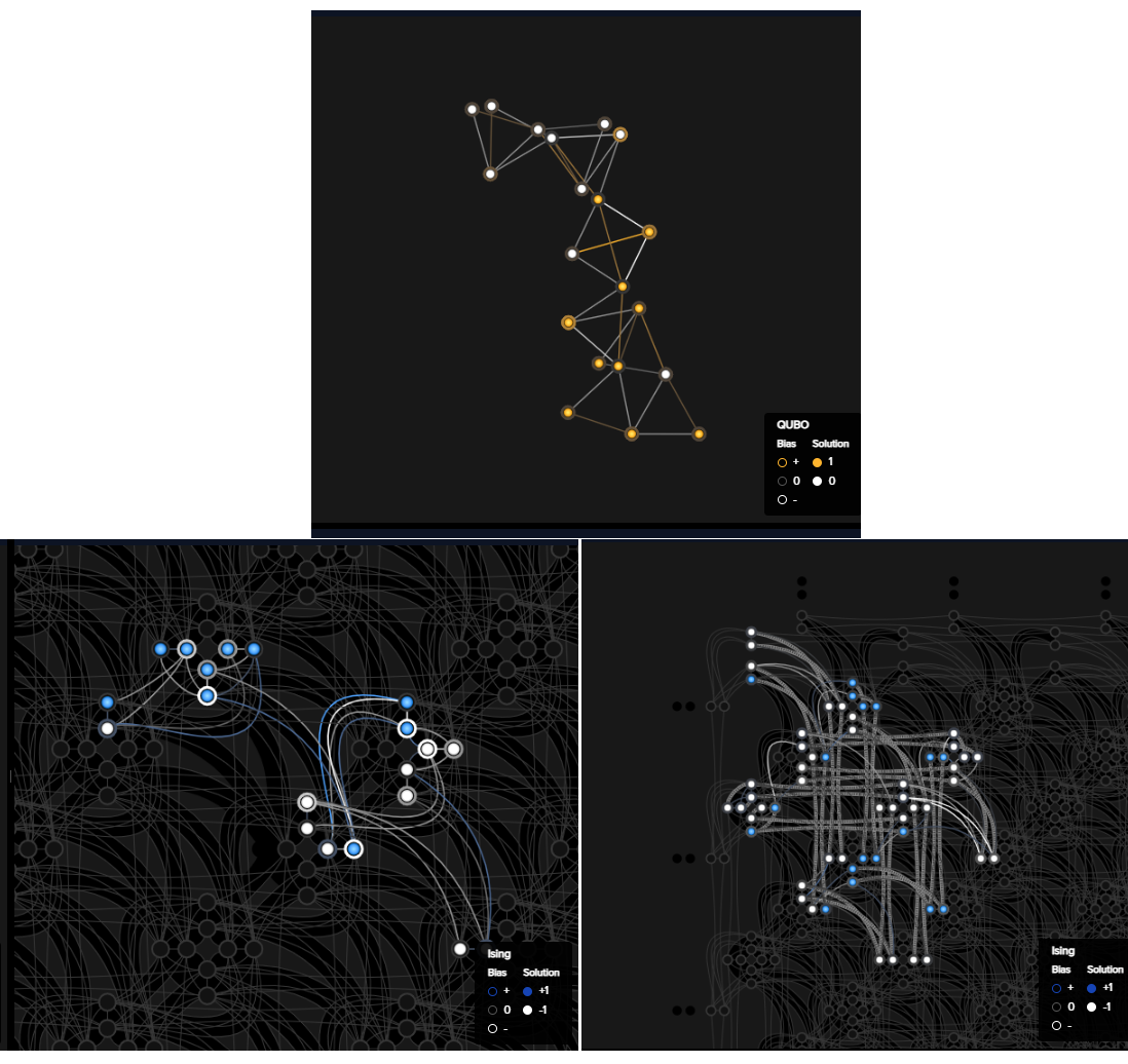
Graph of two replications of the \(z = \overline{b} (ac + ad + \overline{c}\overline{d})\) circuit (top centre), a standard embedding (bottom-left), and a clique-embedding (bottom-right).#
Short chains of a few qubits generally enable good quality solutions: as shown in the table above, for a two-replications circuit the ratio of ground states is similar for both embedding methods.
The BQM representing ten replications of the \(z = \overline{b} (ac + ad + \overline{c}\overline{d})\) circuit has over 100 variables. Typically, minor embeddings for dense graphs require longer chains than those of sparse graphs; for this problem the clique embedding needed chains of up to 11 qubits versus the standard embedding’s chains of 2 qubits. Depending on the problem, such chains may degrade the solution, as is the case here.
>>> bqm = circuit_bqm(10)
>>> for sampler in samplers.values():
...    sampleset = sampler.sample(bqm, num_reads=5000, return_embedding=True)
...    chain_len = max(len(x) for x in sampleset.info["embedding_context"]["embedding"].values())
...    print("Maximum chain length: {}".format(chain_len))
...    dwave.inspector.show(sampleset)
Maximum chain length: 2
Maximum chain length: 11
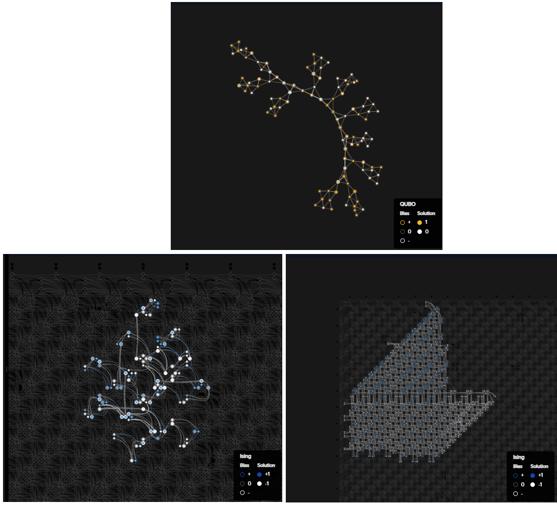
Graph of ten replications of the \(z = \overline{b} (ac + ad + \overline{c}\overline{d})\) circuit (top centre), an embedding (bottom-left), a clique-embedding (bottom-right).#
The Using the Problem Inspector example demonstrates how the problem inspector can be used to analyze your problem submissions.
Performance Comparison: Embedding Executions#
Algorithmic minor embedding is heuristic: solution results can vary significantly based on the minor embedding found.
The table below compares, for a single random ran_r()
problem of a given size, the ratio of ground states to total samples returned
from the quantum computer over several executions[5] of minor embedding.
The outlier results are bolded.
For each run, the EmbeddingComposite composed
sampler finds and returns a minor embedding for the problem. The returned
embedding is then reused twice by a
FixedEmbeddingComposite composed sampler.
Execution |
Ground-State Ratio [%] |
Chain Length |
|---|---|---|
1 |
10.1, 10.1, 8.9 |
4 |
2 |
25.8, 29.1, 28.4 |
4 |
3 |
24.9, 24.4, 27.9 |
3 |
4 |
14.0, 11.0, 13.6 |
3 |
5 |
38.5, 36.4, 34.5 |
4 |
6 |
15.4, 14.6, 14.5 |
4 |
7 |
43.8, 44.2, 45.1 |
3 |
8 |
15.9, 17.2, 15.3 |
4 |
9 |
31.1, 34.1, 27.1 |
3 |
10 |
15.3, 11.5, 12.1 |
3 |
You can see that each set of three submission of the problem using the same embedding have minor variations in the ground-state ratios. However, the variation across minor-embeddings of the same problem can be significant. Consequently, for some applications it can be beneficial to run the minor-embedding multiple times and select the best embedding.