Vertex Cover#
This example solves a few small examples of a known graph problem, minimum vertex cover. A vertex cover is a set of vertices such that each edge of the graph is incident with at least one vertex in the set. A minimum vertex cover is the vertex cover of smallest size.
The purpose of this example is to help a new user to submit a problem to a D-Wave system using Ocean tools with little configuration or coding. Other examples demonstrate more advanced steps that might be needed for complex problems.
Example Requirements#
The code in this example requires that your development environment have Ocean software and be configured to access SAPI, as described in the Initial Set Up section.
Solution Steps#
Section Workflow Steps: Formulation and Sampling describes the problem-solving workflow as consisting of two main steps: (1) Formulate the problem as an objective function in a supported model and (2) Solve your model with a D-Wave solver.
In this example, a function in Ocean software handles both steps. Our task is mainly to select the sampler used to solve the problem.
Formulate the Problem#
The real-world application for this example might be a network provider’s routers interconnected by fiberoptic cables or traffic lights in a city’s intersections. It is posed as a graph problem; here, the five-node star graph shown below. Intuitively, the solution to this small example is obvious — the minimum set of vertices that touch all edges is node 0, but the general problem of finding such a set is NP hard.
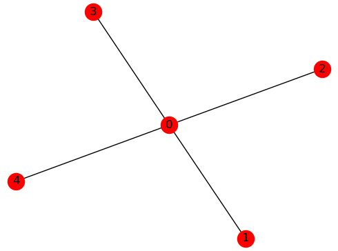
A five-node star graph.#
First, run the code snippet below to create a star graph where node 0 is hub to four other nodes. The code uses NetworkX, which is part of your dwave_networkx or dwave-ocean-sdk installation.
>>> import networkx as nx
>>> s5 = nx.star_graph(4)
Solve the Problem by Sampling#
For small numbers of variables, even your computer’s CPU can solve minimum vertex covers quickly. This example demonstrates how to solve the problem both classically on your CPU and on the quantum computer.
Solving Classically on a CPU#
Before using the D-Wave system, it can sometimes be helpful to test code locally. Here, select one of Ocean software’s test samplers to solve classically on a CPU. Ocean’s dimod provides a sampler that simply returns the BQM’s value for every possible assignment of variable values.
>>> from dimod.reference.samplers import ExactSolver
>>> sampler = ExactSolver()
The next code lines use Ocean’s dwave_networkx
to produce a BQM for our s5 graph and solve it on our selected sampler. In other
examples the BQM is explicitly created but the Ocean tool used here abstracts the
BQM: given the problem graph it returns a solution to a BQM it creates internally.
>>> import dwave_networkx as dnx
>>> print(dnx.min_vertex_cover(s5, sampler))
[0]
Solving on a D-Wave System#
Now use a sampler from Ocean software’s
dwave-system to solve on a
D-Wave system. In addition to DWaveSampler, use
EmbeddingComposite, which maps
unstructured problems to the graph structure of the selected sampler, a process known as
minor-embedding: our problem star graph must be mapped to the QPU’s numerically
indexed qubits.
Note
The code below sets a sampler without specifying SAPI parameters. Configure a default solver as described in Configuring Access to Leap’s Solvers to run the code as is, or see dwave-cloud-client to access a particular solver by setting explicit parameters in your code or environment variables.
>>> from dwave.system import DWaveSampler, EmbeddingComposite
>>> sampler = EmbeddingComposite(DWaveSampler())
>>> print(dnx.min_vertex_cover(s5, sampler))
[0]
Additional Problem Graphs#
The figure below shows another five-node (wheel) graph.

A five-node wheel graph.#
The code snippet below creates a new graph and solves on a D-Wave system.
>>> w5 = nx.wheel_graph(5)
>>> print(dnx.min_vertex_cover(w5, sampler))
[0, 1, 3]
Note that the solution found for this problem is not unique; for example, [0, 2, 4] is also a valid solution.
>>> print(dnx.min_vertex_cover(w5, sampler))
[0, 2, 4]
The figure below shows a ten-node (circular-ladder) graph.
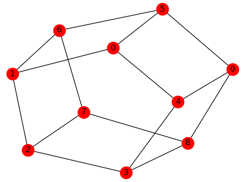
A ten-node circular-ladder graph.#
The code snippet below replaces the problem graph and submits twice to the D-Wave system for solution, producing two of the possible valid solutions.
>>> c5 = nx.circular_ladder_graph(5)
>>> print(dnx.min_vertex_cover(c5, sampler))
[0, 2, 3, 6, 8, 9]
>>> print(dnx.min_vertex_cover(c5, sampler))
[1, 3, 4, 5, 7, 9]
Summary#
In the terminology of Ocean Software Stack, Ocean tools moved the original problem through the following layers:
Application: an example application might be placing limited numbers of traffic-monitoring equipment on routers in a telecommunication network. Such problems can be posed as graphs.
Method: graph mapping. Many different real-world problems can be formulated as instances of classified graph problems. Some of these are hard and the best currently known algorithms for solution may not scale well. Quantum computing might provide better solutions. In this example, vertex cover is a hard problem that can be solved on D-Wave systems.
Sampler API: the Ocean tool internally builds a BQM with lowest values (“ground states”) that correspond to a minimum vertex cover and uses our selected sampler to solve it.
Sampler: classical
ExactSolverand thenDWaveSampler.Compute resource: first a local CPU then a D-Wave system.