Boolean AND Gate#
This example solves a simple problem of a Boolean AND gate on a D-Wave system to demonstrate programming the underlying hardware more directly; in particular, minor-embedding a chain.
Other examples demonstrate more advanced steps that are typically needed for solving actual problems.
Example Requirements#
The code in this example requires that your development environment have Ocean software and be configured to access SAPI, as described in the Initial Set Up section.
Solution Steps#
Section Workflow Steps: Formulation and Sampling describes the problem-solving workflow as consisting of two main steps: (1) Formulate the problem as an objective function in a supported model and (2) Solve your model with a D-Wave solver.
This example mathematically formulates the BQM and uses Ocean tools to solve it on a D-Wave quantum computer.
Formulate the AND Gate as a BQM#
Ocean tools can automate the representation of logic gates as a BQM, as demonstrated in the Multiple-Gate Circuit example. The Boolean NOT Gate example presents a mathematical formulation of a BQM for a Boolean gate in detail. This example briefly repeats the steps of mathematically formulating a BQM while adding details on the underlying physical processes.
A D-Wave quantum processing unit (QPU) is a chip with interconnected qubits; for example, an Advantage QPU has over 5000 qubits connected in a Pegasus topology. Programming it consists mostly of setting two inputs:
Qubit bias weights: control the degree to which a qubit tends to a particular state.
Qubit coupling strengths: control the degree to which two qubits tend to the same state.
The biases and couplings define an energy landscape, and the D-Wave quantum computer seeks the minimum energy of that landscape. Once you express your problem in a formulation[1] such that desired outcomes have low energy values and undesired outcomes high energy values, the D-Wave system solves your problem by finding the low-energy states.
This example uses another binary quadratic model (BQM), the computer-science equivalent of the Ising model, the QUBO: given \(M\) variables \(x_1,...,x_N\), where each variable \(x_i\) can have binary values \(0\) or \(1\), the system tries to find assignments of values that minimize
where \(q_i\) and \(q_{i,j}\) are configurable (linear and quadratic) coefficients. To formulate a problem for the D-Wave system is to program \(q_i\) and \(q_{i,j}\) so that assignments of \(x_1,...,x_N\) also represent solutions to the problem.
AND as a Penalty Function#
This example represents the AND operation, \(z \Leftrightarrow x_1 \wedge x_2\), where \(x_1, x_2\) are the gate’s inputs and \(z\) its output, using a penalty function:
This penalty function represents the AND gate in that for assignments of variables that match valid states of the gate, the function evaluates at a lower value than assignments that would be invalid for the gate. Therefore, when the D-Wave system minimizes a BQM based on this penalty function, it finds those assignments of variables that match valid gate states.
You can verify that this penalty function represents the AND gate in the same way as was done in the Boolean NOT Gate example. See the D-Wave Problem-Solving Handbook for more information about penalty functions in general, and penalty functions for representing Boolean operations in particular.
Formulating the Problem as a QUBO#
For this example, the penalty function is quadratic, and easily reordered in the familiar QUBO formulation:
where \(z=x_3\) is the AND gate’s output, \(x_1, x_2\) the inputs, linear coefficients are \(q_1=3\), and quadratic coefficients are \(q_{1,2}=1, q_{1,3}=-2, q_{2,3}=-2\). The coefficients matrix is,
See the Getting Started with the D-Wave System and D-Wave Problem-Solving Handbook books for more information about formulating problems as QUBOs.
The line of code below sets the QUBO coefficients for this AND gate.
>>> Q = {('x1', 'x2'): 1, ('x1', 'z'): -2, ('x2', 'z'): -2, ('z', 'z'): 3}
Solve the Problem by Sampling (Automated Minor-Embedding)#
For reference, first solve with the same steps used in the Boolean NOT Gate example.
Again use sampler DWaveSampler from Ocean software’s
dwave-system and
its EmbeddingComposite composite to minor-embed
the unstructured problem (variables \(x_1\), :math`x_2`, and :math`z`) on the sampler’s graph structure (the
QPU’s numerically indexed qubits).
The next code sets up a D-Wave system as the sampler.
Note
The code below sets a sampler without specifying SAPI parameters. Configure a default solver as described in Configuring Access to Leap’s Solvers to run the code as is, or see dwave-cloud-client to access a particular solver by setting explicit parameters in your code or environment variables.
>>> from dwave.system import DWaveSampler, EmbeddingComposite
>>> sampler = DWaveSampler()
>>> sampler_embedded = EmbeddingComposite(sampler)
As before, ask for 5000 samples.
>>> sampleset = sampler_embedded.sample_qubo(Q, num_reads=5000,
...                                          label='SDK Examples - AND Gate')
>>> print(sampleset)
  x1 x2  z energy num_oc. chain_b.
0  0  1  0    0.0    1812      0.0
1  1  0  0    0.0     645      0.0
2  1  1  1    0.0     862      0.0
3  0  0  0    0.0    1676      0.0
5  1  0  0    0.0       1 0.333333
6  1  1  1    0.0       1 0.333333
4  0  1  1    1.0       3      0.0
['BINARY', 7 rows, 5000 samples, 3 variables]
Almost all the returned samples from this execution represent valid value assignments for an AND gate, and minimize (are low-energy states of) the BQM.
Note that lines 5 and 6 of output from this execution show samples that seem
identical to lines 1 and 2 (but with non-zero values in the rightmost column,
chain_b.). The next section addresses that.
Understanding Minor-Embedding#
This section looks more closely into minor-embedding. Above and in the Boolean NOT Gate
example, dwave-system
EmbeddingComposite composite abstracted the minor-embedding.
Minor-Embedding a NOT Gate#
For simplicity, first return to the NOT gate. The Boolean NOT Gate example found that a NOT gate can be represented by a BQM in QUBO form with the following coefficients:
>>> Q_not = {('x', 'x'): -1, ('x', 'z'): 2, ('z', 'x'): 0, ('z', 'z'): -1}
Minor embedding maps the two problem variables x and z to the indexed qubits of the D-Wave QPU. Here, do this mapping yourself.
The next line of code looks at the nodelist property of the sampler. Select
the first node, which on a QPU is a qubit, and print its adjacent nodes, which
are the qubits it is coupled to.
>>> sampler.nodelist[0]
30
>>> print(sampler.adjacency[sampler.nodelist[0]])
{2985, 2955, 45, 2970, 2940, 31}
For the Advantage system the above code ran on in this particular execution,
you see that the first available qubit, 30, is adjacent to qubit 31
and a few others.
You can map the NOT problem’s two linear coefficients (coefficients of the
\(-1x\) and \(-1z\) terms) and single quadratic coefficient (coefficient
of the \(2xz\) term) to \(q_1=q_2=-1\) biases applied to the Advantage’s
qubits 30 and 31 and a \(q_{1,2}=2\) coupling strength applied to
coupler [30, 31]. The figure below shows this embedding of the NOT gate
onto an Advantage QPU.
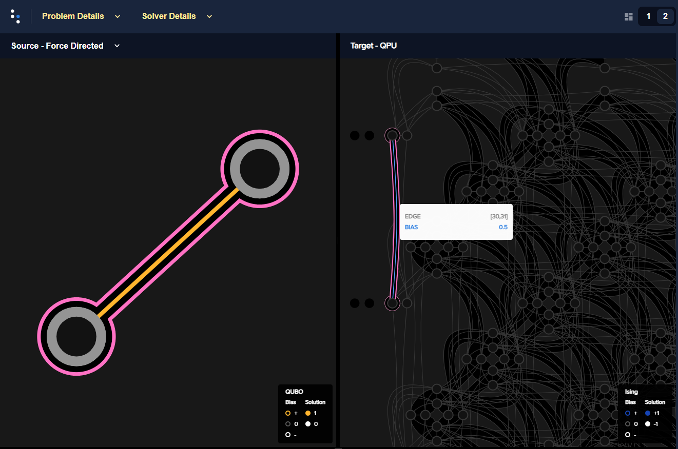
A NOT gate minor embedded onto an Advantage QPU. Variables \(x,z\)
(left) are minor-embedded to qubits 30 and 31 (right). This
visualization is produced by Ocean’s dwave-inspector tool.#
Notice that coupling strength is BIAS 0.5 above: as explained in the
system documentation,
the QPU can be viewed as minimizing the Ising model (see Ising footnote
above), with linear biases setting the amplitudes of magnetic fields applied
to qubits and quadratic biases the strength of coupling between qubits. While
QUBOs are more convenient to work with for some problems, Ocean converts
problems submitted to a QPU to equivalent Ising models, producing the
\(J_{1,2}\) bias of 0.5 for the [30, 31] coupler shown above (and
, not shown, zero \(h_1=h_2\) biases on the two qubits):
>>> dimod.qubo_to_ising(Q_not)
({'x': 0.0, 'z': 0.0}, {('x', 'z'): 0.5}, -0.5)
The following code uses the FixedEmbeddingComposite
composite to manually minor-embed the problem on this Advantage QPU.[2]
>>> from dwave.system import FixedEmbeddingComposite
>>> sampler_embedded = FixedEmbeddingComposite(sampler, {"x": [30], "z": [31]})
>>> print(sampler_embedded.adjacency["x"])
{'z'}
As in the Boolean NOT Gate example, most the results from 5000 samples are valid states of a NOT gate, with complementary values for \(x\) and \(z\).
>>> sampleset = sampler_embedded.sample_qubo(Q_not, num_reads=5000,
...                                          label='SDK Examples - AND Gate')
>>> print(sampleset)
   x  z energy num_oc. chain_.
0  0  1   -1.0    2264     0.0
1  1  0   -1.0    2733     0.0
2  0  0    0.0       2     0.0
3  1  1    0.0       1     0.0
['BINARY', 4 rows, 5000 samples, 2 variables]
The crucial point to understand in this subsection is that you cannot map the
set of your problem’s variables to a set of arbitrary qubits. Quadratic models
have interactions between some pairs of the variables and those require the
existence of couplers between the qubits representing such variable pairs;
because the graph of a QPU is not fully connected, not all qubits are coupled.
For interacting variables \(x, z\) of the NOT gate, the selection of qubit
30 for variable \(x\) severely limits the possible choices of qubits
that can represent variable \(z\).
From NOT to AND to Larger Problems#
The BQM for a NOT gate, \(-x -z + 2xz\), can be represented by a fully connected \(K_2\) graph: its linear coefficients are weights of the two connected nodes with the single quadratic coefficient the weight of its connecting edge.
The BQM for an AND gate, \(3z + x_1x_2 - 2x_1z - 2x_2z\), needs a \(K_3\) graph.
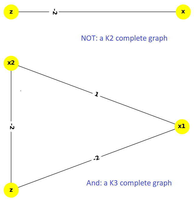
NOT gate \(K_2\) complete graph (top) versus AND gate \(K_3\) complete graph (bottom.)#
In the previous subsection, to minor-embed a \(K_2\) graph on a QPU, you selected an arbitrary qubit (for simplicity, the first listed) and could then select as the second any of the qubits coupled to the first. Minor-embedding a \(K_3\) graph on a D-Wave QPU is less straightforward.
Consider trying to expand the minor embedding you found for the NOT gate above
to the AND gate. On the same QPU, map \(x_1\) and \(x_2\) to the qubits
used before, 30 and 31, respectively. For \(z\) you now need a third
qubit coupled to both:
>>> print(sampler.adjacency[30])
{2985, 2955, 45, 2970, 2940, 31}
>>> print(sampler.adjacency[31])
{32, 46, 3150, 3120, 3165, 30, 3135}
Qubit 30 is coupled to 5 additional qubits and qubit 31 is coupled to 6,[3]
but none common to both. Because each qubit is coupled to a limited set of other
qubits, only a minority of coupled qubits are also coupled in common to a
third qubit.
In this case, a more successful selection for variables \(x_1\) and
\(x_2\) is the set of qubits 30 and 2985:
>>> print(sampler.adjacency[30])
{2985, 2955, 45, 2970, 2940, 31}
>>> print(sampler.adjacency[2985])
{195, 165, 135, 2986, 45, 180, 150, 120, 2970, 30}
Both these qubits are also coupled to qubit 45 and 2970.
The figure below shows a minor embedding of the AND gate onto an Advantage QPU.
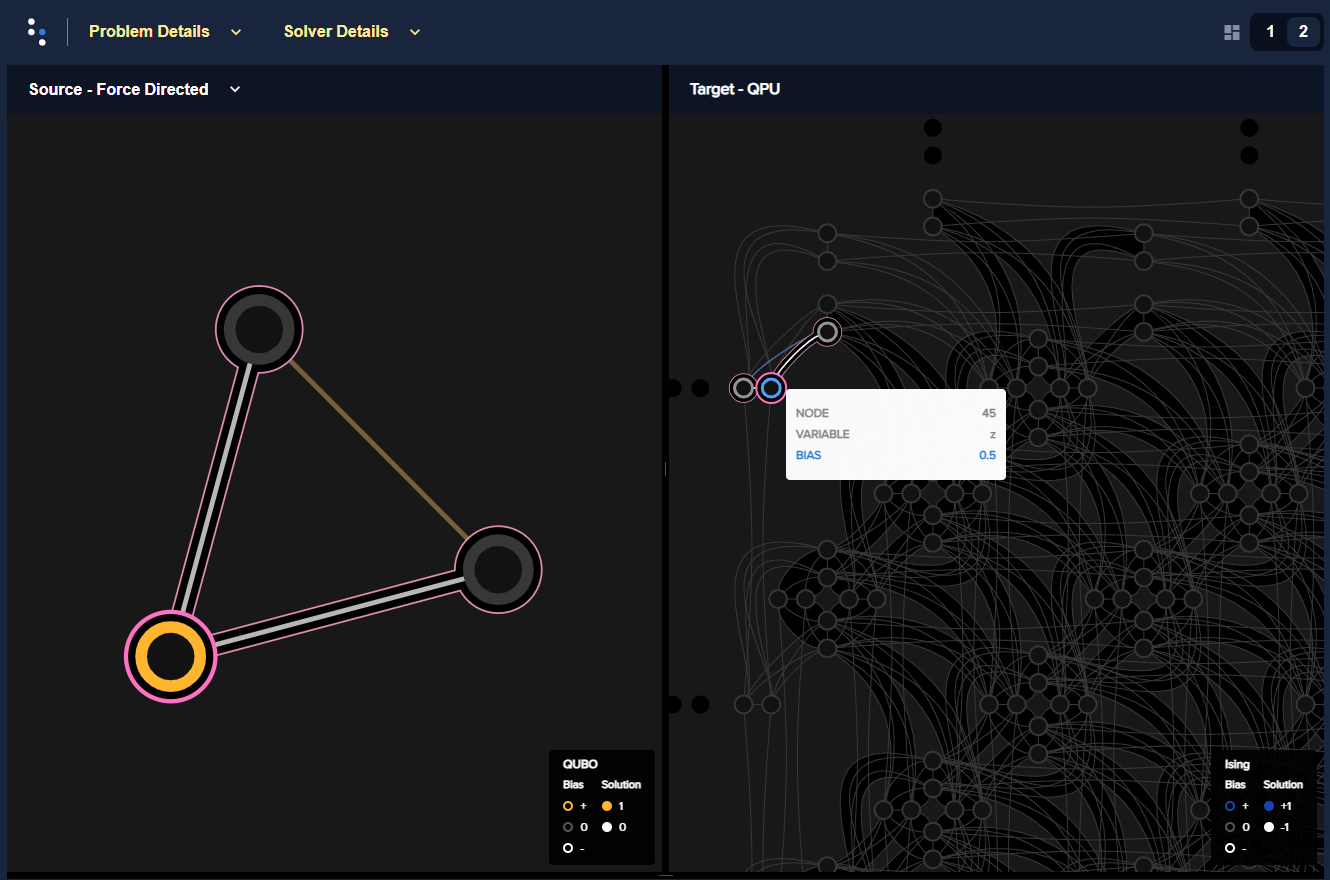
An AND gate minor embedded onto an Advantage QPU. Variables \(x_1, x_2, z\)
(left) are minor-embedded to qubits 30, 2985 and 45 (right).#
Can you always make a successful selection of qubits such that all your problem’s variables are mapped to qubits with couplings that can represent all the problem’s interactions? Such one-to-one embeddings, with each graph node represented by a single qubit, are called native embeddings. The largest clique you can embed natively on the Pegasus topology is a \(K_4\). Larger cliques such as \(K_5\), as well as large, non-clique (“sparse”) graphs, require chaining qubits.
Chains#
To understand how chaining qubits overcomes the problem of sparse connectivity, consider minor embedding the triangular \(K_3\) graph below into two target graphs, one sparser than the other. The graphic below shows two such embeddings: the \(K_3\) graph is mapped on the left to a fully-connected graph of four nodes (a \(K_4\) complete graph ) and on the right to a sparser graph, also of four nodes. For the left-hand embedding, you can choose any mapping between \(a, b, c\) and \(0, 1, 2, 3\); here \(a, b, c\) are mapped to \(2, 0, 1\), respectively. For the right-hand embedding, however, no choice of just three target nodes suffices. The same \(2, 0, 1\) target nodes leaves \(b\) disconnected from \(c\). Chaining target nodes \(0\) and \(3\) to represent node \(b\) makes use of both the connection between \(0\) to \(2\) and the connection between \(3\) and \(1\).
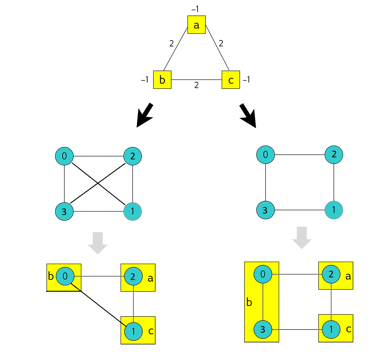
Embedding a triangular graph into fully connected and sparse four-node graphs.#
On QPUs, chaining qubits is accomplished by setting the strength of their connecting couplers negative enough to strongly correlate the states of the chained qubits; if at the end of most anneals these qubits are in the same classical state, representing the same binary value in the objective function, they are in effect acting as a single variable.
The strength of the coupler between qubits 0 and 3, which represents variable
\(b\), must be set to correlate the qubits strongly, so that in most
solutions they have a single value for \(z\). (Remember the output in the
Solve the Problem by Sampling (Automated Minor-Embedding) section with its lines 5 and 6? The chain_b.
column stands for “chain breaks”, which is when qubits in a chain take different
values.)
The previous subsection showed that if you mapped the AND problem’s variables
\(x_1\) and \(x_2\) to qubits 30 and 31, respectively, on the
QPU used before, you could not find a single qubit coupled to both for variable
\(z\). But notice, for example, that qubit 30 (representing \(x_1\))
is coupled to qubit 45 and qubit 31 (representing \(x_2\)) is coupled
to qubit 46. You can represent variable \(z\) as a chain of qubits
45 and 46, which are coupled:
>>> (45, 46) in sampler.edgelist
True
>>> sampler_embedded = FixedEmbeddingComposite(sampler, {"x1": [30], "x2": [31], "z": [45, 46]})
>>> sampleset = sampler_embedded.sample_qubo(Q, num_reads=5000,
...                                          label='SDK Examples - AND Gate')
>>> print(sampleset)
  x1 x2  z energy num_oc. chain_b.
0  0  1  0    0.0    1522      0.0
1  1  1  1    0.0    1219      0.0
2  0  0  0    0.0    1080      0.0
3  1  0  0    0.0    1163      0.0
4  1  0  1    1.0       6      0.0
5  1  1  0    1.0       6      0.0
6  0  1  1    1.0       2      0.0
7  0  1  1    1.0       2 0.333333
['BINARY', 8 rows, 5000 samples, 3 variables]
The figure below shows this minor embedding of the AND gate onto this Advantage QPU.
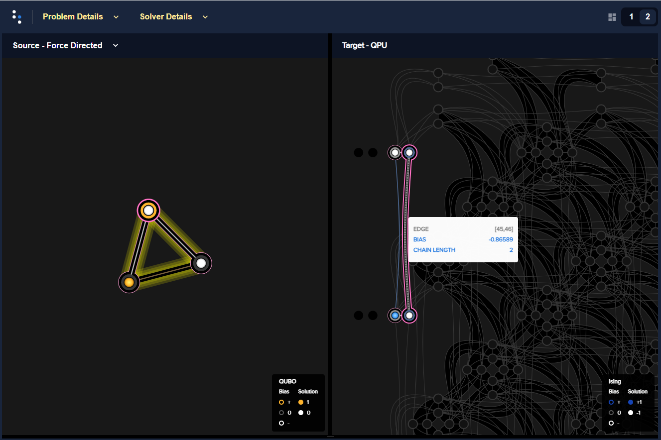
An AND gate minor embedded onto an Advantage QPU. Variables \(x_1, x_2, z\)
(left) are minor-embedded to qubits 30, 31 and chain [45, 46] (right).#
Chain Strength#
For illustrative purposes, this subsection purposely weakens the
chain strength (strength of the coupling
between qubits 45 and 46, which represent variable \(z\)).
In the previous subsection, the chain strength, which by default is set by the
uniform_torque_compensation() function,
was close to 1.
>>> print(round(sampleset.info['embedding_context']['chain_strength'], 3))
0.866
The following code explicitly sets chain strength to a lower value of 0.25.
Consequently, the two qubits are less strongly correlated and the result is that
many returned samples represent invalid states for an AND gate.
Note
The next code requires the use of Ocean’s dwave-inspector tool.
>>> import dwave.inspector
>>> sampleset = sampler_embedded.sample_qubo(Q, num_reads=5000,
...                                          chain_strength=0.25,
...                                          label='SDK Examples - AND Gate')
>>> print(sampleset)
  x1 x2  z energy num_oc. chain_b.
  x1 x2  z energy num_oc. chain_b.
0  0  1  0    0.0    1046      0.0
1  1  1  1    0.0     401      0.0
2  0  0  0    0.0    1108      0.0
3  1  0  0    0.0     885      0.0
4  1  0  1    1.0     917 0.333333
5  0  1  1    1.0     643 0.333333
['BINARY', 6 rows, 5000 samples, 3 variables]
In this case, as above, you are likely to see many samples with broken chains
(these have non-zero values in the chain_b. column) and calling the
problem inspector shows these:
>>> dwave.inspector.show(sampleset)
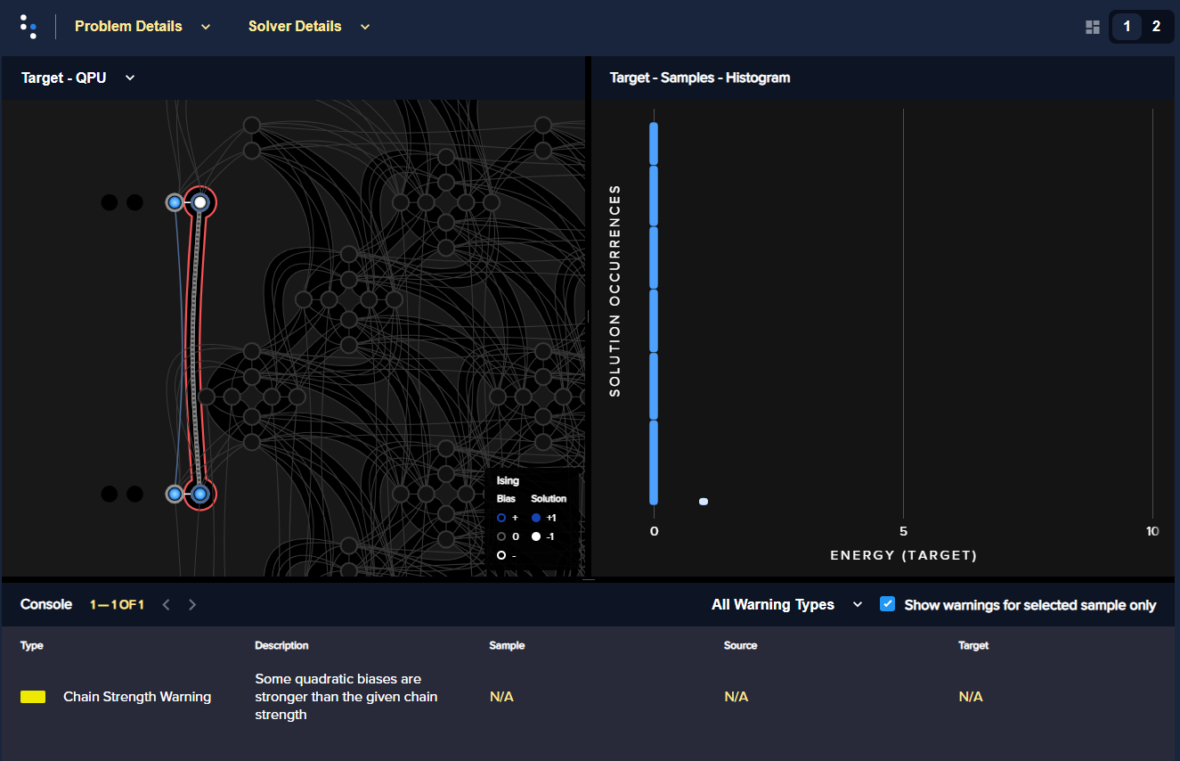
An AND gate minor embedded onto an Advantage QPU with a low chain strength. For the selection of a result with a high energy (right), the broken chain is highlighted in red (left), with one of the chain’s qubits returning 1 and the other -1.#