Using the Framework#
This section helps you quickly use a provided reference sampler to solve arbitrary-sized problems and then shows you how to build (hybrid) workflows using provided components.
Reference Hybrid Sampler: Kerberos#
dwave-hybrid includes a reference example sampler built using the framework: Kerberos is a dimod-compatible hybrid asynchronous decomposition sampler that enables you to solve problems of arbitrary structure and size. It finds best samples by running in parallel tabu search, simulated annealing, and D-Wave subproblem sampling on problem variables that have high-energy impact.
The example below uses Kerberos to solve a large QUBO.
>>> import dimod
>>> from hybrid.reference.kerberos import KerberosSampler
>>> with open('../problems/random-chimera/8192.01.qubo') as problem:
...     bqm = dimod.BinaryQuadraticModel.from_coo(problem)
>>> len(bqm)
8192
>>> solution = KerberosSampler().sample(bqm, max_iter=10, convergence=3)
>>> solution.first.energy
-4647.0
Building Workflows#
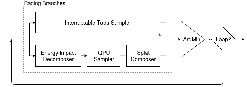
As shown in the Overview section, you build hybrid solvers by arranging components such as samplers in a workflow.
Building Blocks#
The basic components—building blocks—you use are based on the
Runnable class: decomposers, samplers, and composers. Such components
input a set of samples, a SampleSet, and output updated
samples. A State associated with such an iteration of a component holds
the problem, samples, and optionally additional information.
The following example demonstrates a simple workflow that uses just one
Runnable, a sampler representing the classical tabu search algorithm,
to solve a problem (fully classically, without decomposition). The example
solves a small problem of a triangle graph of nodes identically coupled. An
initial State of all-zero samples is set as a starting point. The
solution, new_state, is derived from a single iteration of the
TabuProblemSampler Runnable.
>>> import dimod
>>> # Define a problem
>>> bqm = dimod.BinaryQuadraticModel.from_ising({}, {'ab': 0.5, 'bc': 0.5, 'ca': 0.5})
>>> # Set up the sampler with an initial state
>>> sampler = TabuProblemSampler(tenure=2, timeout=5)
>>> state = State.from_sample({'a': 0, 'b': 0, 'c': 0}, bqm)
>>> # Sample the problem
>>> new_state = sampler.run(state).result()
>>> print(new_state.samples)
    a   b   c  energy  num_occ.
0  +1  -1  -1    -0.5         1
['SPIN', 1 rows, 1 samples, 3 variables]
Flow Structuring#
The framework provides classes for structuring workflows that use the
“building-block” components. As shown in the Overview section,
you can create a branch of Runnable classes; for example
decomposer | sampler | composer, which delegates part of a problem to a
sampler such as a D-Wave quantum computer.
The following example shows a branch comprising a decomposer, local Tabu
solver, and a composer. A 10-variable binary quadratic model is decomposed by
the energy impact of its variables into a 6-variable subproblem to be sampled
twice. An initial state of all -1 values is set using the utility function
min_sample().
>>> import dimod           # Create a binary quadratic model
>>> bqm = dimod.BinaryQuadraticModel({t: 0 for t in range(10)},
...                                  {(t, (t+1) % 10): 1 for t in range(10)},
...                                  0, 'SPIN')
>>> branch = (EnergyImpactDecomposer(size=6, min_gain=-10) |
...           TabuSubproblemSampler(num_reads=2) |
...           SplatComposer())
>>> new_state = branch.next(State.from_sample(min_sample(bqm), bqm))
>>> print(new_state.subsamples)
    4   5   6   7   8   9  energy  num_occ.
0  +1  -1  -1  +1  -1  +1    -5.0         1
1  +1  -1  -1  +1  -1  +1    -5.0         1
['SPIN', 2 rows, 2 samples, 6 variables]
Such Branch classes can be run in parallel using the
RacingBranches class. From the outputs of these parallel branches,
ArgMin selects a new current sample. And instead of a single iteration
on the sample set, you can use the Loop to iterate a set number of
times or until a convergence criteria is met.
This example of Racing Branches solves a binary quadratic model by iteratively producing best samples. It employs both tabu search on the entire problem and a D-Wave quantum computer on subproblems. In addition to building-block components such as employed above, this example also uses infrastructure classes to manage the decomposition and parallel running of branches.

Racing Branches#
import dimod
import hybrid

# Construct a problem
bqm = dimod.BinaryQuadraticModel({}, {'ab': 1, 'bc': -1, 'ca': 1}, 0, dimod.SPIN)

# Define the workflow
iteration = hybrid.RacingBranches(
    hybrid.InterruptableTabuSampler(),
    hybrid.EnergyImpactDecomposer(size=2)
    | hybrid.QPUSubproblemAutoEmbeddingSampler()
    | hybrid.SplatComposer()
) | hybrid.ArgMin()
workflow = hybrid.LoopUntilNoImprovement(iteration, convergence=3)

# Solve the problem
init_state = hybrid.State.from_problem(bqm)
final_state = workflow.run(init_state).result()

# Print results
print("Solution: sample={.samples.first}".format(final_state))
Flow Refining#
The framework enables quick modification of work flows to improve solutions and performance. For example, after verifying the Racing Branches workflow above on its small problem, you might make a series of modifications such as the examples below to better fit it to problems with large numbers of variables.
Configure a decomposition window that moves down a fraction of problem variables, ordered from highest to lower energy impact, and submit those subproblems to a D-Wave quantum computer while tabu searches globally. This example submits 50-variable subproblems on up to 15% of the total variables.
# Redefine the workflow: a rolling decomposition window
subproblem = hybrid.EnergyImpactDecomposer(size=50, rolling_history=0.15)
subsampler = hybrid.QPUSubproblemAutoEmbeddingSampler() | hybrid.SplatComposer()

iteration = hybrid.RacingBranches(
    hybrid.InterruptableTabuSampler(),
    subproblem | subsampler
) | hybrid.ArgMin()

workflow = hybrid.LoopUntilNoImprovement(iteration, convergence=3)
Instead of sequentially producing a sample per subproblem, a further modification might be to process all the subproblems in parallel and merge the returned samples. Here the
EnergyImpactDecomposeris iterated until it raises aEndOfStream()exception when it reaches 15% of the variables, and then all the 50-variable subproblems are submitted to the D-Wave quantum computer in parallel. Subsamples returned by the QPU are disjoint in variables, so we can easily reduce them all to a single subsample, which is then merged with the input sample usingSplatComposer:
# Redefine the workflow: parallel subproblem solving for a single sample
subproblem = hybrid.Unwind(
    hybrid.EnergyImpactDecomposer(size=50, rolling_history=0.15)
)

# Helper function to merge subsamples in place
def merge_substates(_, substates):
    a, b = substates
    return a.updated(subsamples=hybrid.hstack_samplesets(a.subsamples, b.subsamples))

# Map QPU sampling over all subproblems, then reduce subsamples by merging in place
subsampler = hybrid.Map(
    hybrid.QPUSubproblemAutoEmbeddingSampler()
) | hybrid.Reduce(
    hybrid.Lambda(merge_substates)
) | hybrid.SplatComposer()
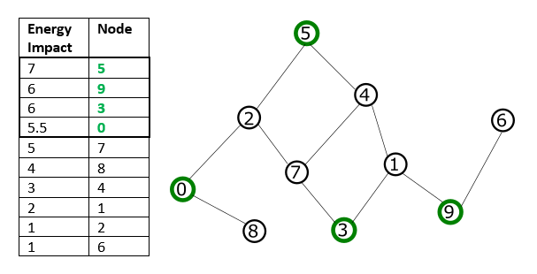
Change the criterion for selecting subproblems. By default, the variables are selected by maximal energy impact but selection can be better tailored to a problem’s structure.
For example, for binary quadratic model representing the problem graph shown in the Traversal by Energy Impact graphic, if you select a subproblem size of four, these nodes selected by descending energy impact are not directly connected (no shared edges, and might not represent a local structure of the problem).

Traversal by Energy Impact#
Configuring a mode of traversal such as breadth-first (BFS) or priority-first selection (PFS) can capture features that represent local structures within a problem.
# Redefine the workflow: subproblem selection
subproblem = hybrid.Unwind(
    hybrid.EnergyImpactDecomposer(size=50, rolling_history=0.15, traversal='bfs'))
These two selection modes are shown in the Traversal by BFS or PFS graphic. BFS starts with the node with maximal energy impact, from which its graph traversal proceeds to directly connected nodes, then nodes directly connected to those, and so on, with graph traversal ordered by node index. In PFS, graph traversal selects the node with highest energy impact among unselected nodes directly connected to any already selected node.

Traversal by BFS or PFS#
Additional Examples#
Tailoring State Selection#
The next example tailors a state selector for a sampler that does some
post-processing and can alert upon suspect samples. Sampler output modified by
ellipses (”…”) for readability is shown below for an Ising model of a triangle
problem with zero biases and interactions all equal to 0.5. The first of three
State classes is flagged as problematic using the info
field:
[{...,'samples': SampleSet(rec.array([([0, 1, 0], 0., 1)], ..., ['a', 'b', 'c'], {'Postprocessor': 'Excessive chain breaks'}, 'SPIN')},
{...,'samples': SampleSet(rec.array([([1, 1, 1], 1.5, 1)], ..., ['a', 'b', 'c'], {}, 'SPIN')},
{...,'samples': SampleSet(rec.array([([0, 0, 0], 0., 1)], ..., ['a', 'b', 'c'], {}, 'SPIN')}]
This code snippet defines a metric for the key argument in ArgMin:
def preempt(si):
    if 'Postprocessor' in si.samples.info:
        return(math.inf)
    else:
        return(si.samples.first.energy)
Using the defined key on the above input, ArgMin finds the
state with the lowest energy (zero) excluding the flagged state (which also has
energy of zero):
>>> ArgMin(key=preempt).next(states)
{'problem': BinaryQuadraticModel({'a': 0.0, 'b': 0.0, 'c': 0.0}, {('a', 'b'): 0.5, ('b', 'c'): 0.5, ('c', 'a'): 0.5},
0.0, Vartype.SPIN), 'samples': SampleSet(rec.array([([0, 0, 0], 0., 1)],
dtype=[('sample', 'i1', (3,)), ('energy', '<f8'), ('num_occurrences', '<i4')]), ['a', 'b', 'c'], {}, 'SPIN')}
Parallel Sampling#
The code snippet below uses Map to run a tabu search on
two states in parallel.
>>> Map(TabuProblemSampler()).run(States(
        State.from_sample({'a': 0, 'b': 0, 'c': 1}, bqm1),
        State.from_sample({'a': 1, 'b': 1, 'c': 0}, bqm2)))
>>> _.result()
[{'samples': SampleSet(rec.array([([-1, -1,  1], -0.5, 1)], dtype=[('sample', 'i1', (3,)),
 ('energy', '<f8'), ('num_occurrences', '<i4')]), ['a', 'b', 'c'], {}, 'SPIN'),
 'problem': BinaryQuadraticModel({'a': 0.0, 'b': 0.0, 'c': 0.0}, {('a', 'b'): 0.5, ('b', 'c'): 0.5,
 ('c', 'a'): 0.5}, 0.0, Vartype.SPIN)},
 {'samples': SampleSet(rec.array([([ 1,  1, -1], -1., 1)], dtype=[('sample', 'i1', (3,)),
 ('energy', '<f8'), ('num_occurrences', '<i4')]), ['a', 'b', 'c'], {}, 'SPIN'),
 'problem': BinaryQuadraticModel({'a': 0.0, 'b': 0.0, 'c': 0.0}, {('a', 'b'): 1, ('b', 'c'): 1,
 ('c', 'a'): 1}, 0.0, Vartype.SPIN)}]
Logging and Execution Information#
You can see detailed execution information by setting the level of logging.
The package supports logging levels TRACE, DEBUG, INFO, WARNING, ERROR, and
CRITICAL in ascending order of severity. By default, logging level is set to
ERROR. You can select the logging level with environment variable
DWAVE_HYBRID_LOG_LEVEL.
For example, on a Windows operating system, set this environment variable to INFO level as:
set DWAVE_HYBRID_LOG_LEVEL=INFO
or on a Unix-based system as:
DWAVE_HYBRID_LOG_LEVEL=INFO
The previous example above might output something like the following:
>>> print("Solution: sample={s.samples.first}".format(s=solution))
2018-12-10 15:18:30,634 hybrid.flow INFO Loop Iteration(iterno=0, best_state_quality=-3.0)
2018-12-10 15:18:31,511 hybrid.flow INFO Loop Iteration(iterno=1, best_state_quality=-3.0)
2018-12-10 15:18:35,889 hybrid.flow INFO Loop Iteration(iterno=2, best_state_quality=-3.0)
2018-12-10 15:18:37,377 hybrid.flow INFO Loop Iteration(iterno=3, best_state_quality=-3.0)
Solution: sample=Sample(sample={'a': 1, 'b': -1, 'c': -1}, energy=-3.0, num_occurrences=1)