Minor-Embedding#
To solve an arbitrarily posed binary quadratic problem directly on a D-Wave
system requires mapping, called minor embedding, to the QPU Topology
of the system’s quantum processing unit (QPU). This preprocessing can be done
by a composed sampler consisting of the
DWaveSampler() and a composite that performs
minor-embedding. (This step is handled automatically by
LeapHybridSampler() and
dwave-hybrid reference samplers.)
For example, a simple two-variable bqm,
might be embedded to two connected qubits, such as 633 and 3603 on an Advantage
system:
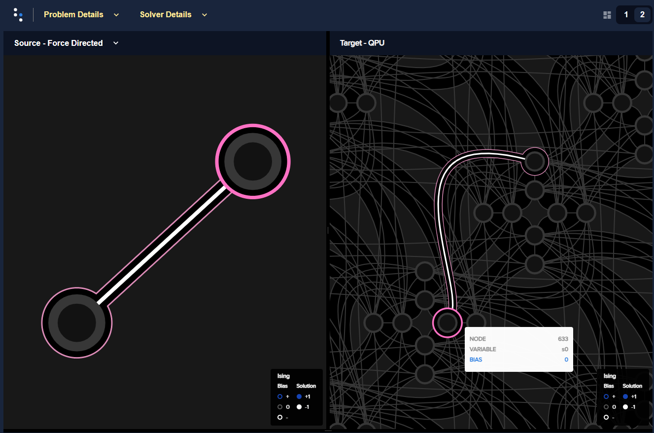
Two-variable problem, shown on the left as a graph, is embedded in two connected qubits on an Advantage, shown on the right against the Pegasus topology. Variable \(s_0\), highlighted in dark magenta, is represented by qubit number 633 and variable \(s_1\) is represented by qubit 3603. (This and similar images in this section are generated by Ocean’s problem inspector tool.#
In the Advantage Pegasus topology, most qubits are connected to fifteen
other qubits, so other valid minor-embeddings might be 633 for \(s_0\)
and 634 for \(s_1\) or 4628 for \(s_0\) and 1749 for
\(s_1\).
Chains#
Larger problems often require chains because the QPU topology is not fully connected. For example, a \(K_5\) graph is not native to the Pegasus topology, meaning that the following five-variable bqm with a clique (fully-connected) \(K_5\) graph cannot be represented by five qubits on an Advantage QPU.
>>> import dimod
>>> bqm = dimod.generators.doped(1, 5)
>>> bqm.add_linear_from({v: 1 for v in bqm.variables})
Instead, at least one variable is represented by a chain of physical qubits, as in this minor-embedding:
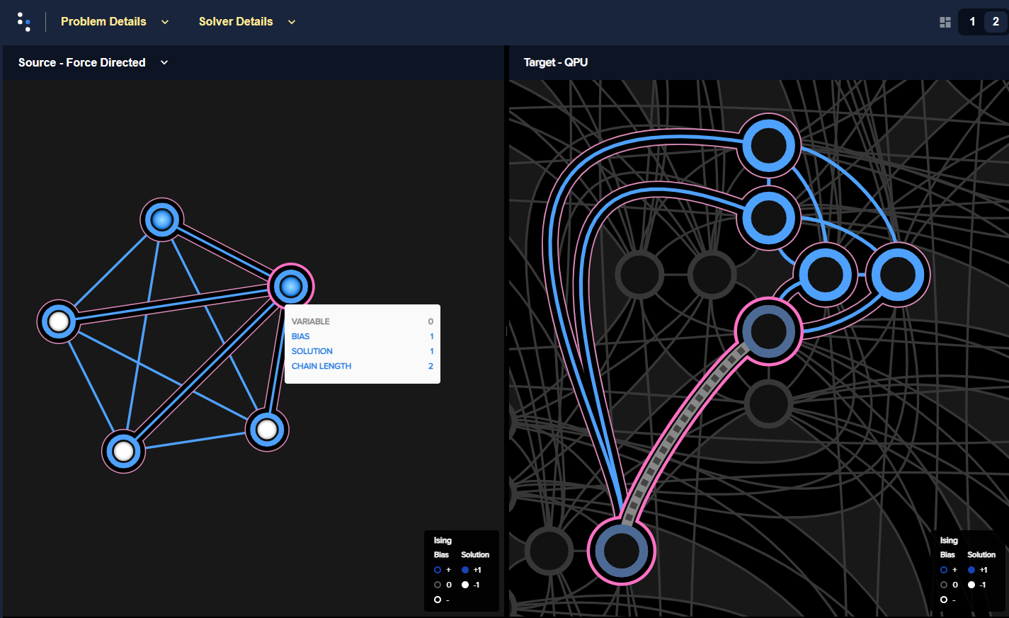
Five-variable \(K_5\) fully-connected problem, shown on the left as a graph, is embedded in six qubits on an Advantage, shown on the right against the Pegasus topology. Variable 0, highlighted in dark magenta, is represented by two qubits, 1975 and 4840.#
The minor-embedding above was derived from the hueristic used by
EmbeddingComposite() on the working graph of
an Advantage selected by DWaveSampler():
>>> from dwave.system import DWaveSampler, EmbeddingComposite, FixedEmbeddingComposite
>>> sampler = EmbeddingComposite(DWaveSampler())
Other qubits might have been chosen; for example,
>>> sampler = FixedEmbeddingComposite(DWaveSampler(),
...     embedding={0: [4408, 2437], 1: [4333], 2: [4348], 3: [2497], 4: [2512]})
intentionally sets the embedding shown below to represent this same \(K_5\) graph:
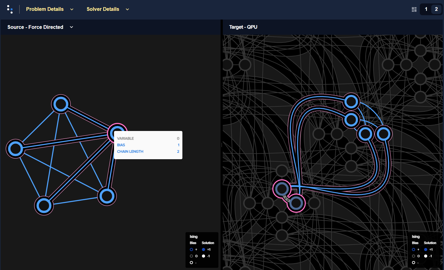
Five-variable \(K_5\) fully-connected problem, shown on the left as a graph, is embedded in six qubits on an Advantage, shown on the right against the Pegasus topology. Variable 0, highlighted in dark magenta, is represented by two qubits, 4408 and 2437.#
Chain Strength#
For a chain of qubits to represent a variable, all its constituent qubits must return the same value for a sample. This is accomplished by setting a strong coupling to the edges connecting these qubits. That is, for the qubits in a chain to be likely to return identical values, the coupling strength for their connecting edges must be strong compared to the coupling with other qubits that influence non-identical outcomes.
The \(K_5\) BQM has ten ground states (best solutions). These are shown below—solved by brute-force stepping through all possible configurations of values for the variables—with ground-state energy -3.0:
>>> print(dimod.ExactSolver().sample(bqm).lowest())
   0  1  2  3  4 energy num_oc.
0 +1 +1 -1 -1 -1   -3.0       1
1 -1 +1 +1 -1 -1   -3.0       1
2 +1 -1 +1 -1 -1   -3.0       1
3 -1 -1 +1 +1 -1   -3.0       1
4 -1 +1 -1 +1 -1   -3.0       1
5 +1 -1 -1 +1 -1   -3.0       1
6 -1 -1 -1 +1 +1   -3.0       1
7 -1 -1 +1 -1 +1   -3.0       1
8 -1 +1 -1 -1 +1   -3.0       1
9 +1 -1 -1 -1 +1   -3.0       1
['SPIN', 10 rows, 10 samples, 5 variables]
These solutions are states in which two variables are assigned one value and the remaining three variables the complementary value; for example two are \(-1\) and three \(+1\) as shown below.
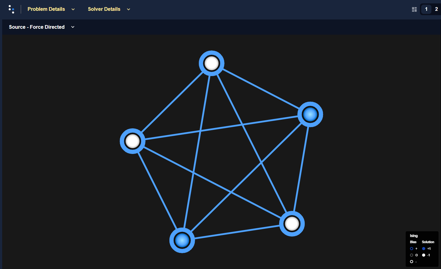
Ground state of the five-variable \(K_5\) fully-connected problem.#
A typical submission of the problem to a quantum computer, using the same minor-embedding as the previous subsection and the default chain strength, returned all the ground states, with these solutions constituting over 90% of the returned samples.
>>> sampleset = sampler.sample(bqm, num_reads=1000)
>>> print(sampleset.lowest())
    0  1  2  3  4 energy num_oc. chain_.
0  -1 +1 +1 -1 -1   -3.0      69     0.0
1  +1 -1 -1 +1 -1   -3.0     115     0.0
2  +1 -1 -1 -1 +1   -3.0      95     0.0
3  +1 -1 +1 -1 -1   -3.0      84     0.0
4  -1 -1 -1 +1 +1   -3.0     116     0.0
5  -1 -1 +1 +1 -1   -3.0      99     0.0
6  -1 -1 +1 -1 +1   -3.0      91     0.0
7  +1 +1 -1 -1 -1   -3.0      71     0.0
8  -1 +1 -1 +1 -1   -3.0      98     0.0
9  -1 +1 -1 -1 +1   -3.0      95     0.0
10 +1 -1 -1 +1 -1   -3.0       1     0.2
['SPIN', 11 rows, 934 samples, 5 variables]
The default chain strength is set by the
uniform_torque_compensation() function:
>>> print(round(sampleset.info['embedding_context']['chain_strength'], 3))
2.828
Resubmitting with a much lower chain strength produced less satisfactory results (only ~10% of returned samples are ground states).
>>> sampleset = sampler.sample(bqm, num_reads=1000, chain_strength=1)
>>> print(sampleset.lowest())
   0  1  2  3  4 energy num_oc. chain_.
0 -1 +1 +1 -1 -1   -3.0      12     0.0
1 +1 -1 -1 +1 -1   -3.0      13     0.0
2 +1 -1 -1 -1 +1   -3.0      13     0.0
3 +1 -1 +1 -1 -1   -3.0      16     0.0
4 -1 -1 -1 +1 +1   -3.0       6     0.0
5 -1 -1 +1 +1 -1   -3.0      10     0.0
6 -1 -1 +1 -1 +1   -3.0      17     0.0
7 +1 +1 -1 -1 -1   -3.0      17     0.0
8 -1 +1 -1 +1 -1   -3.0      10     0.0
9 -1 +1 -1 -1 +1   -3.0       7     0.0
['SPIN', 10 rows, 121 samples, 5 variables]
Many of the remaining ~90% of returned samples have “broken chains”, meaning qubits of a chain did not have identical values due to insufficiently strong coupling compared to quadratic coefficients of interactions (of the variable the chain represented) with other variables.
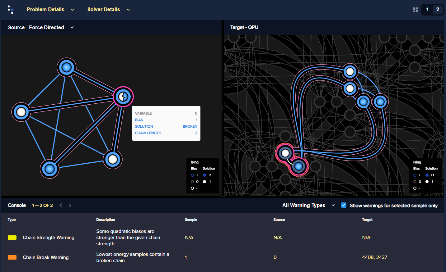
Five-variable \(K_5\) fully-connected problem is embedded in six qubits on an Advantage using a low chain strength. Variable 0, highlighted in dark magenta, is represented by two qubits, numbers 2437 and 4408. The displayed solution has a broken chain: qubit 4408 returned a value of \(-1\) (represented by a white dot) while qubit 2347 returned a value of \(+1\) (a blue dot). The logical representation of the problem, on the left, shows a half-white, half-blue dot to represent a value based on a broken chain.#
For information on handling embedding and chains, see the following documentation:
Boolean AND Gate, Multiple-Gate Circuit, and Using the Problem Inspector examples
Show through some simple examples how to embed and set chain strength.
minorminer tool
Is the hueristic used by common Ocean embedding composites.
problem inspector tool
Visualizes embeddings.
dwave-system Composites section
Provides embedding composites
dwave-system Embedding section
Describes chain-related functionality.