Models: BQM, CQM, QM, Others

Constrained Versus Unconstrained

Many real-world problems include constraints. For example, a routing problem might limit the number of airplanes on the ground at an airport and a scheduling problem might require a minimum interval between shifts.

Constrained models such as ConstrainedQuadraticModel can support constraints by encoding both an objective and its set of constraints, as models or in symbolic form.

Unconstrained quadratic models are used to submit problems to samplers such as D-Wave quantum computers1 and some hybrid quantum-classical samplers2.

When using such samplers to handle problems with constraints, you typically formulate the constraints as penalties: see Getting Started with D-Wave Solvers. (Constrained models, such as the ConstrainedQuadraticModel, can support constraints natively.)

1

D-Wave quantum computers accept unconstrained binary quadratic models, such as quadratic unconstrained binary optimization (QUBO) models: binary because variables are represented by qubits that return two states and quadratic because polynomial terms of two variables can be represented by pairs of coupled qubits.

2

Some hybrid quantum-classical samplers accept constrained and non-binary models; for example, a quadratic model with an integer variable that must be smaller than some configured value.

Supported Models

• Binary Quadratic Models

  The binary quadratic model (BQM) class, BinaryQuadraticModel, encodes Ising and quadratic unconstrained binary optimization (QUBO) models used by samplers such as D-Wave’s quantum computers.

  For an introduction to BQMs, see Concepts: Binary Quadratic Models. For the BQM class, its attributes and methods, see the BQM reference documentation.

• Constrained Quadratic Model

  The constrained quadratic model (CQM) class, ConstrainedQuadraticModel, encodes a quadratic objective and possibly one or more quadratic equality and inequality constraints.

  For an introduction to CQMs, see Constrained Quadratic Models. For descriptions of the CQM class and its methods, see Constrained Quadratic Model.

• Quadratic Models

  The quadratic model (QM) class, QuadraticModel, encodes polynomials of binary, integer, and discrete variables, with all terms of degree two or less.

  For an introduction to QMs, see Concepts: Quadratic Models. For the QM class, its attributes and methods, see the QM reference documentation.

• Discrete Quadratic Models

  The discrete quadratic model (BQM) class, DiscreteQuadraticModel, encodes polynomials of discrete variables, with all terms of degree two or less.

  For an introduction to DQMs, see Concepts: Discrete Quadratic Models. For the DQM class, its attributes and methods, see DQM reference documentation.

• Higher-Order Models

  dimod provides some Higher-Order Composites and functionality such as reducing higher-order polynomials to BQMs.

Model Construction

dimod provides a variety of model generators. These are especially useful for testing code and learning.

See examples of using QPU solvers and Leap hybrid solvers on these models in Ocean documentation’s Getting Started examples and the dwave-examples GitHub repository.

Typically you construct a model when reformulating your problem, using such techniques as those presented in D-Wave’s system documentation’s Problem-Solving Handbook.

CQM Example: Using a dimod Generator

This example creates a CQM representing a knapsack problem of ten items.

>>> cqm = dimod.generators.random_knapsack(10)

CQM Example: Symbolic Formulation

This example constructs a CQM from symbolic math, which is especially useful for learning and testing with small CQMs.

>>> x = dimod.Binary('x')
>>> y = dimod.Integer('y')
>>> cqm = dimod.CQM()
>>> objective = cqm.set_objective(x+y)
>>> cqm.add_constraint(y <= 3) 
'...'

For very large models, you might read the data from a file or construct from a NumPy array.

BQM Example: Using a dimod Generator

This example generates a BQM from a fully-connected graph (a clique) where all linear biases are zero and quadratic values are uniformly selected -1 or +1 values.

>>> bqm = dimod.generators.random.ran_r(1, 7)

BQM Example: Python Formulation

For learning and testing with small models, construction in Python is convenient.

The maximum cut problem is to find a subset of a graph’s vertices such that the number of edges between it and the complementary subset is as large as possible.

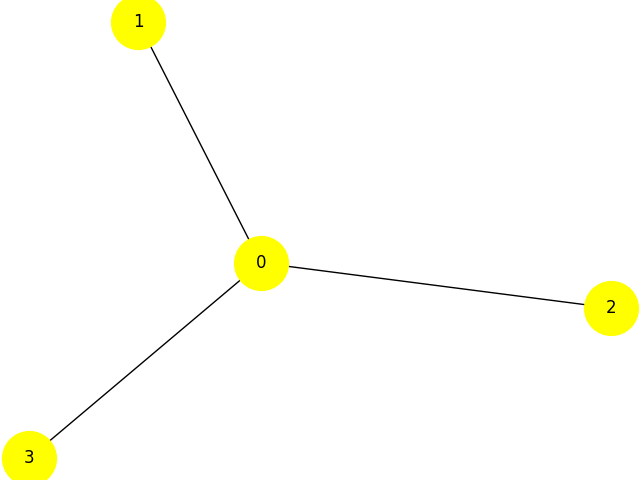
Star graph with four nodes.

The dwave-examples Maximum Cut example demonstrates how such problems can be formulated as QUBOs:

\[\begin{split}Q = \begin{bmatrix} -3 & 2 & 2 & 2\\ 0 & -1 & 0 & 0\\ 0 & 0 & -1 & 0\\ 0 & 0 & 0 & -1 \end{bmatrix}\end{split}\]

>>> qubo = {(0, 0): -3, (1, 1): -1, (0, 1): 2, (2, 2): -1,
...         (0, 2): 2, (3, 3): -1, (0, 3): 2}
>>> bqm = dimod.BQM.from_qubo(qubo)

BQM Example: Construction from NumPy Arrays

For performance, especially with very large BQMs, you might read the data from a file using methods, such as from_file() or from NumPy arrays.

This example creates a BQM representing a long ferromagnetic loop with two opposite non-zero biases.

>>> import numpy as np
>>> linear = np.zeros(1000)
>>> quadratic = (np.arange(0, 1000), np.arange(1, 1001), -np.ones(1000))
>>> bqm = dimod.BinaryQuadraticModel.from_numpy_vectors(linear, quadratic, 0, "SPIN")
>>> bqm.add_quadratic(0, 10, -1)
>>> bqm.set_linear(0, -1)
>>> bqm.set_linear(500, 1)
>>> bqm.num_variables
1001

QM Example: Interaction Between Integer Variables

This example constructs a QM with an interaction between two integer variables.

>>> qm = dimod.QuadraticModel()
>>> qm.add_variables_from('INTEGER', ['i', 'j'])
>>> qm.add_quadratic('i', 'j', 1.5)

Data Structure

Quadratic models are implemented with an adjacency structure in which each variable tracks its own linear bias and its neighborhood. The figure below shows the graph and adjacency representations for an example BQM,

\[E(x) = .5 x_0 - 3 x_1 - x_0 x_1 + x_0 x_2 + 2 x_0 x_3 + x_2 x_3\]

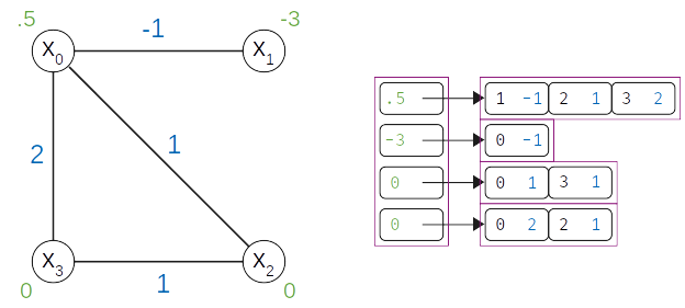
Adjacency structure of a 4-variable binary quadratic model.