Introduction

Nonlinear programming (NLP) is the process of solving an optimization problem where some of the constraints are not linear equalities and/or the objective function is not a linear function. Such optimization problems are pervasive in business and logistics: inventory management, scheduling employees, equipment delivery, and many more.

Nonlinear Models

dwave-optimization enables you to formulate the nonlinear models needed for such industrial optimization problems. The model can then be submitted to the Leap^TM service’s quantum-classical hybrid nonlinear-program solver to find good solutions.

Examples of problems suited to such solution methods are resource routing, scheduling, allocation, and job-shop scheduling.

Successful implementation, as for any solver, requires following some best practices in formulating your model.

Symbols

Nonlinear models can be mapped to a directed acyclic graph. The model’s symbols—decision variables, intermediate variables, constants, and mathematical operations—are represented as nodes in the graph while the flow of operations upon these symbols are represented as the graph’s edges.

A nonlinear model as a directed acyclic graph.

Consider an illustrative problem of finding the minimum of a function of an integer variable, the polynomial \(y = i^2 - 4i\).

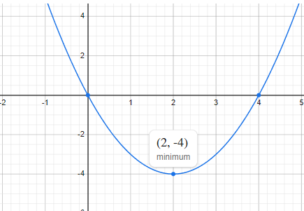
Minimum point of a simple polynomial, \(y = i^2 - 4i\).

The dwave-optimization package can formulate the problem as nonlinear model as follows:

>>> from dwave.optimization import Model
...
>>> model = Model()
>>> i = model.integer(lower_bound=-5, upper_bound=5)
>>> c = model.constant(4)
>>> y = i**2 - c*i
>>> model.minimize(y)

The code above has the following elements:

• i is a IntegerVariable symbol, typically constructed with the integer() method, that represents a single integer of values between \(-5\) and \(+5\). It is a decision variable: to find the minimum of the polynomial, a solver must assign values to decision variable i such that the objective function of this model is minimized.

• c is a Constant symbol that represents a single invariable value, \(4\), which is the linear coefficient multiplying \(i\) in the polynomial. This type of symbol is used as input to mathematical operations but its value is never updated by a solver.

• y is an intermediate symbol used for convenience to formulate the model in a human-readable way. It is fully determined by other symbols—the i and c symbols—and so implicitly constrained. A solver must update y if it updates i, to a value fully determined by the value it selected to assign to i.

• The Min symbol is a mathematical operation on inputs from other symbols. In this model, it generates the objective function.

The directed acyclic graph below illustratively represents the model for minimizing polynomial \(y = i^2 - 4i\).

An directed acyclic graph that illustrates one way of representing the model for minimizing polynomial \(y = i^2 - 4i\). The package’s to_networkx() method generates the graph that actually represents the model.

The package provides various symbols that enable you to select those most suited to an efficient formulation of your model.

States

States represent assignments of values to a symbol. For example, symbol \(k\), defined as an IntegerVariable of size \(2 \times 3\), might have states [[1, 1, 2], [4, 5, 5]] and [[1, 1, 3], [4, 5, 5]]. Such states, which might be returned from a solver in response to a submission that requested two results, represent two assignments that differ in one element of the array (element \(j_{0,2}\)), as is typical at the end of an iterative solution process.

The solutions to nonlinear models you submit to a Leap hybrid nonlinear-program solver are states of the model’s decision variables. For example, the state of symbol i in the model above for the simple polynomial, \(y = i^2 - 4i\).

The dwave-optimization package enables you to set the states of symbols in a model. You can sets states for two purposes:

• Setting initial states for the solver. For some problems you might have estimates or guesses of solutions, and by providing to the solver, as part of your problem submission, such assignments of decision variables as an initial state of the model, you may accelerate the solution.

• Testing and developing your models.

The following code sets states for the i decision variable of the model formulated above for the simple polynomial: for states 0 to 4, it assigns values 0 to 4. It then prints the resulting value of the model’s objective function for each state.

>>> with model.lock():
...     model.states.resize(5)
...     for j in range(5):
...         i.set_state(j, [j])
...     for j in range(5):
...         print(f"For state {j}, i={i.state(j)} results in objective {model.objective.state(j)}")
For state 0, i=0.0 results in objective 0.0
For state 1, i=1.0 results in objective -3.0
For state 2, i=2.0 results in objective -4.0
For state 3, i=3.0 results in objective -3.0
For state 4, i=4.0 results in objective 0.0

The code above selects a symbol by label (’i’); however, you can also set states for symbols of a model without using labels.

>>> with model.lock():
...     for symbol in model.iter_decisions():
...         symbol.set_state(0, [2])
...     assert model.objective.state(0) == -4

This process of iterating through a model to select symbols of various types (decision variables, constraints, etc) is helpful when model construction is separated from model-instance solution, for example in application code or when using the package’s model generators.

Constructing Models

Typically, you construct your model by instantiating decision-variable symbols (“primitives”), using such model methods as integer() and disjoint_lists(), and constants (constant()).

The example below, uses the integer() method to instantiate an IntegerVariable symbol.

>>> from dwave.optimization import Model
...
>>> model = Model()
>>> i = model.integer(100, lower_bound=0, upper_bound=20)

These decision-variable and constant symbols form the “root” of the directed acyclic graph.

An directed acyclic graph that shows a single primitive, decision variable \(i\), an IntegerVariable.

Operations on these symbols, create new symbols, which form the model’s full directed acyclic graph. The Sum symbol, for example, sums the 100 integer elements of the \(1 \times 100\)-shaped IntegerVariable \(i\).

>>> sum_i = i.sum()

An directed acyclic graph that shows a primitive, decision variable \(i\), an IntegerVariable, and \(sum_i\), a Sum symbol.

You can access these symbols by iterating on the model’s symbols.

>>> with model.lock():
...     for symbol in model.iter_symbols():
...         print(f"Symbol {type(symbol)} is node {symbol.topological_index()}")
Symbol <class 'dwave.optimization.symbols.IntegerVariable'> is node 0
Symbol <class 'dwave.optimization.symbols.Sum'> is node 1

Typically, you add symbols to the model through mathematical operations between symbols. The code below adds a symbol that checks that only one of the 100 values assigned to symbol \(i\) is a nonzero positive integer.

>>> max_i = i.max()
>>> one_nozero = (sum_i == max_i).sum()

An directed acyclic graph that shows a primitive, decision variable \(i\), an IntegerVariable, and additional mathematical-operation symbols.

>>> symbols = {}
>>> one_one = 100*[0]
>>> with model.lock():
...     for symbol in model.iter_symbols():
...         symbols[symbol.topological_index()] = symbol
...     last_symbol = max(symbols.keys())
...     model.states.resize(1)
...     one_one[15] = 1
...     symbols[0].set_state(0, one_one)
...     print(symbols[last_symbol].state(0) == True)
...     one_one[25] = 1
...     symbols[0].set_state(0, one_one)
...     print(symbols[last_symbol].state(0) == False)
True
True

Constructing Good Models

As much as possible, design models along these lines:

1. Use compact matrix operations in your formulations.

   The dwave-optimization package enables you to formulate models using linear-algebra conventions similar to NumPy. Compact matrix formulation are usually more efficient and should be preferred.

2. Exploit the implicit constraints of symbols such as ListVariable, SetVariable, DisjointLists, and DisjointBitSets.

   Typically, solver performance strongly depends on the size of the solution space for your modelled problem: models with smaller spaces of feasible solutions tend to perform better than ones with larger spaces. A powerful way to reduce the feasible-solutions space is by using variables that act as implicit constraints. This is analogous to judicious typing of a variable to meet but not exceed its required assignments: a Boolean variable, x, has a solution space of size 2 (\(\{True, False\}\)) while a finite-precision integer variable, i, might have a solution space of several billion values.

See the formulations used by the package’s model generators and relevant GitHub examples for reference.

Example: Compact Matrix Formulation

Like a large class of real-world problems, optimally loading a truck to convey the most valuable merchandise while not exceeding limitations on carrying weight or allowable volume, can be considered a variation on the well-known knapsack optimization problem. The problem is to maximize the total value of items packed in a knapsack without exceeding its capacity.

Such real-world problems, when formulated mathematically for automated solution, typically include a data-transformation step that provides the weights and values of the problem’s items in some structure. Here, an illustrative problem of just four items is modeled, with weights and values \(30, 10, 40, 20\) and \(10, 20, 30, 40\), respectively, and a maximum capacity of \(30\) for the truck.

For a practical formulation of the knapsack problem, see the code in the knapsack generator.

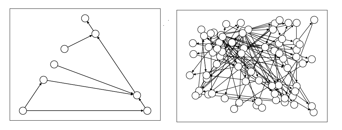
This example compares two formulations of a small truck-loading problem: an intuitive model that represents multiple binary decisions with multiple binary symbols etc. versus a more compact model. The figure below compares the directed acyclic graphs for these two formulations.

Comparison between models using compact matrix operations (left) and less-compact operations (right) in formulation. The less-compact formulation has triple the number of symbols. Graphs are created using the package’s to_networkx() method.

The two tabs below provide the two formulations.

Compact Formulation

The model in this tab is formulated using compact matrix operations.

Instantiate a nonlinear model and add the constant symbols.

>>> model = Model()
>>> weight = model.constant([30, 10, 40, 20])
>>> value = model.constant([10, 20, 30, 40])
>>> capacity = model.constant(30)

Add a binary-array variable for the items: which items should be selected for loading into the truck.

>>> items = model.binary(4)

Add a constraint that the total weight must not exceed the truck’s capacity.

>>> total_weight = items * weight
>>> model.add_constraint(total_weight.sum() <= capacity)

Add the objective (transport as much valuable merchandise as possible):

>>> total_value = items * value
>>> model.minimize(-total_value.sum())

The size of this model is a third of the alternative formulation shown in the second tab:

>>> model.num_nodes()
10

Non-compact Formulation

The model in this tab is formulated using one binary decision variable per item. Each variable and constant adds a node to the directed acyclic graph.

Instantiate a nonlinear model and add the constant symbols. The weight and value of each item is represented by a symbol.

>>> model = Model()
>>> weight0 = model.constant(30)
>>> weight1 = model.constant(10)
>>> weight2 = model.constant(40)
>>> weight3 = model.constant(20)
>>> val0 = model.constant(10)
>>> val1 = model.constant(20)
>>> val2 = model.constant(30)
>>> val3 = model.constant(40)
>>> capacity = model.constant(30)

Add a binary variable for each item: should that item be loaded into the truck (yes or no?).

>>> item0 = model.binary()
>>> item1 = model.binary()
>>> item2 = model.binary()
>>> item3 = model.binary()

Add the constraint on the total weight:

>>> total_weight = item0*weight0 + item1*weight1 + item2*weight2 + item3*weight3
>>> model.add_constraint(total_weight <= capacity)

Add the objective to maximize the transported value:

>>> total_value = item0*val0 + item1*val1 + item2*val2 + item3*val3
>>> model.minimize(-total_value)

The size of this model is triple the alternative formulation shown in the first tab:

>>> model.num_nodes()
29

Compare the two formulations. Prefer compact-matrix formulations for your models.

Example: Implicitly Constrained Symbols

Consider a problem of selecting a route for several destinations with the cost increasing on each leg of the itinerary; for the example formulated below, one can travel through four destinations in any order, one destination per day, with the transportation cost per unit of travel doubling every subsequent day.

The figure below shows four destinations as dots labeled 0 to 3, and plots the least costly (green) and most costly (red) routes.

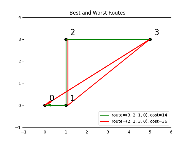
Finding the optimal route between destinations.

The code snippet below defines the cost per leg and the distances between the four destinations, with values chosen for simple illustration.

>>> import numpy as np
...
>>> cost_per_day = [1, 2, 4]
>>> distance_matrix = np.asarray([
...     [0, 1, np.sqrt(10), np.sqrt(34)],
...     [1, 0, 2, np.sqrt(25)],
...     [np.sqrt(10), 3, 0, 4],
...     [np.sqrt(34), np.sqrt(25), 4, 0]])

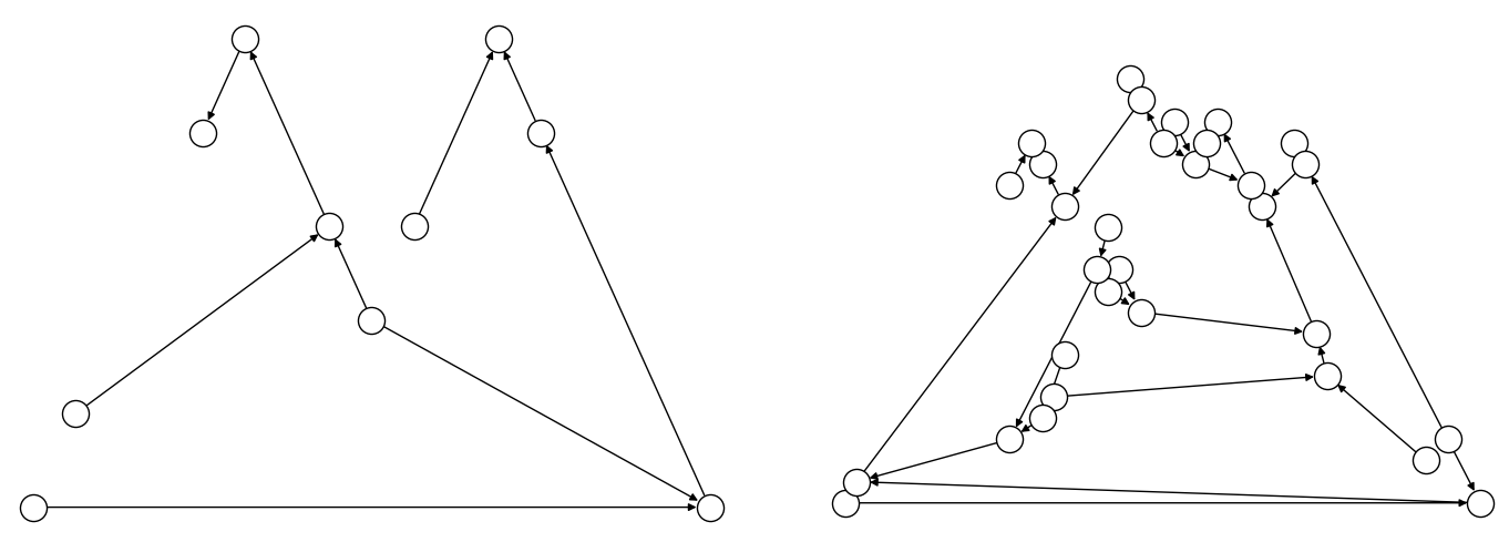
This section compares two formulations of this small routing problem: an intuitive model that uses the generic BinaryVariable symbol to represent decisions on ordering the destinations versus a model that uses the implicitly constrained ListVariable symbol, where the order of destinations is a permutation of values. The figure below compares the directed acyclic graphs for these two formulations.

Comparison between models using explicitly-constrained decision symbol (left) and explicit constrains on a simple binary symbol (right) in formulation. The first formulation has fewer symbols.

It is expected that the more compact model that uses implicit constraints will perform better.

The two tabs below provide the two formulations.

Implicit Constraints

The model in this tab is formulated using the implicitly constrained List symbol.

>>> model = Model()
>>> # Add the constants
>>> cost = model.constant(cost_per_day)
>>> distances = model.constant(distance_matrix)
>>> # Add the decision symbol
>>> route = model.list(4)
>>> # Optimize the objective
>>> model.minimize((cost * distances[route[:-1],route[1:]]).sum())

You can see the objective values for the least and most costly routes as permutations of the \([0, 1, 2, 3]\) list as follows:

>>> with model.lock():
...     model.states.resize(2)
...     route.set_state(0, [3, 2, 1, 0])
...     route.set_state(1, [2, 1, 3, 0])
...     print(int(model.objective.state(0)), int(model.objective.state(1)))
14 36

Explicit Constraints

The model in this tab is formulated using explicit constraints on the generic BinaryVariable symbol.

>>> from dwave.optimization.mathematical import add
...
>>> model = Model()
>>> # Add the problem constants
>>> cost = model.constant(cost_per_day)
>>> distances = model.constant(distance_matrix)

Define constants that are used to formulate the explicit constraints.

>>> one = model.constant(1)
>>> indx_int = model.constant([0, 1, 2, 3])

Add the decision symbol: for each of the itinerary’s four legs, each of the four destinations is represented by a binary variable. If leg 1 should be to destination 2, for example, the value of row 1 is \(False, False, True, False\). This is a representation known as one-hot encoding.

>>> itinerary_loc = model.binary((4, 4))

Add the objective. Here, the indx_int constant converts the binary one-hot variables to an index of the distance matrix.

>>> indx = []
>>> for i in range(distances.shape()[0]):
...     indx.append((itinerary_loc[i,:] * indx_int).sum())
>>> model.minimize(add(*[cost[i]*distances[indx[i], indx[i+1]] for
...     i in range(distances.shape()[0]-1)]))

Add explicit one-hot constraints: summing the columns of the decision variable must give ones because each destination is visited once; summing rows must give ones because each leg visits one destination.

>>> for i in range(distances.shape()[0]):
...     model.add_constraint(itinerary_loc[i, :].sum() <= one)
...     model.add_constraint(one <= itinerary_loc[i,:].sum())
...     model.add_constraint(itinerary_loc[:, i].sum() <= one)
...     model.add_constraint(one <= itinerary_loc[:, i].sum())

You can see the objective cost for the least costly route as follows:

>>> with model.lock():
...     model.states.resize(2)
...     itinerary_loc.set_state(0, [
...         [0, 0, 0, 1],
...         [0, 0, 1, 0],
...         [0, 1, 0, 0],
...         [1, 0, 0, 0]])
...     print(int(model.objective.state(0)))
14

The directed acyclic graph for the implicitly constrained model has few nodes and the model is more efficient.