Introduction#
dwave-inspector provides a graphic interface for examining D-Wave quantum computers’
problems and answers. As described in the
Ocean documentation’s Getting Started,
the D-Wave system solves problems formulated as binary quadratic models (BQM) that are
mapped to its qubits in a process called minor-embedding. Because the way you choose to
minor-embed a problem (the mapping and related parameters) affects solution quality,
it can be helpful to see it.
For example, minor-embedding a problem represented by a \(K_5\) fully-connected graph into an Advantage QPU, with its Pegasus topology, requires representing one of the five variables with a chain of two physical qubits:
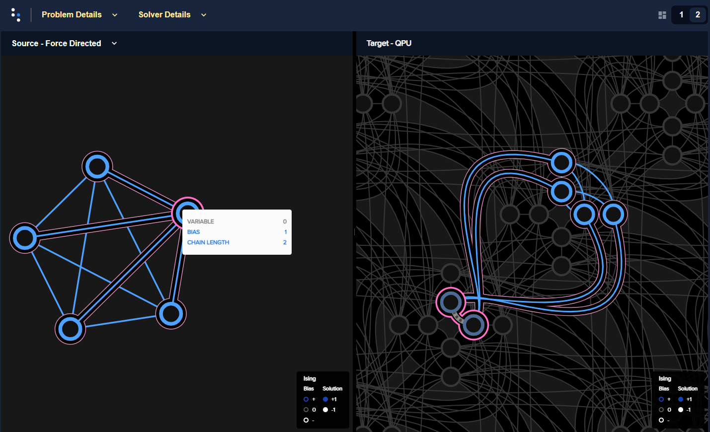
Five-variable \(K_5\) fully-connected problem, shown on the left as a
graph, is embedded in six qubits on an Advantage, shown on the right against
the Pegasus topology. Variable 0, highlighted in dark magenta, is
represented by two qubits, 1975 and 4840 in this particular embedding.#
The problem inspector shows you your chains at a glance: you see lengths, any breakages, and physical layout.
Usage and Examples#
Import the problem inspector to enable it[1] to hook into your problem submissions.
The following examples demonstrate the use of the show() method to visualize
an embedded problem and a
logical problem in your default browser.
Inspecting an Embedded Problem#
This example shows the canonical usage: samples representing physical qubits on a quantum processing unit (QPU).
>>> from dwave.system import DWaveSampler
>>> import dwave.inspector
...
>>> # Get solver
>>> sampler = DWaveSampler(solver=dict(topology__type='pegasus'))
...
>>> # Define a problem (actual qubits depend on the selected QPU's working graph)
>>> h = {}
>>> J = {(2136, 4181): -1, (2136, 2151): -0.5, (2151, 4196): 0.5, (4181, 4196): 1}
>>> all(edge in sampler.edgelist for edge in J)
True
>>> # Sample
>>> response = sampler.sample_ising(h, J, num_reads=100)
...
>>> # Inspect
>>> dwave.inspector.show(response)
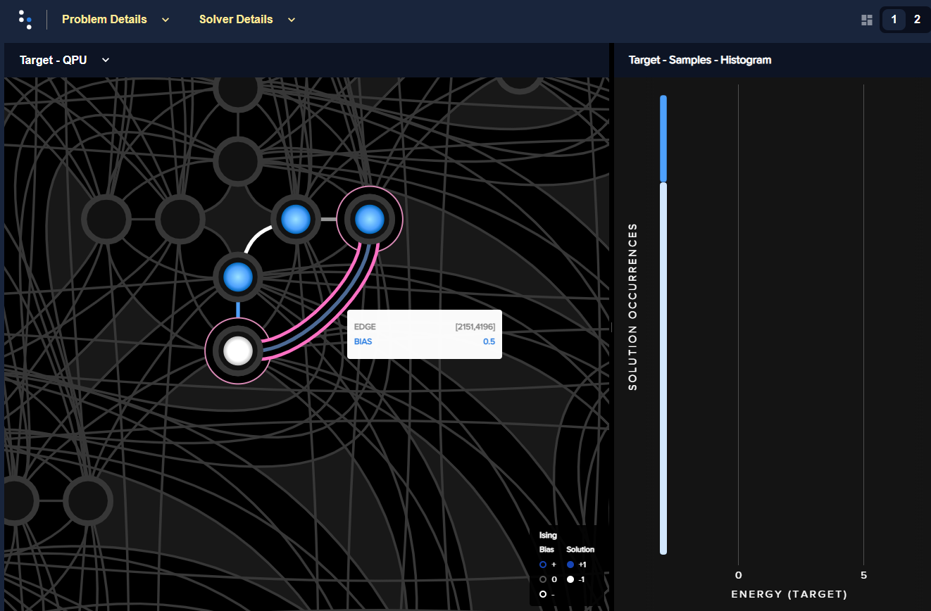
Edge values between qubits 2136, 4181, 2151, and 4196, and the
selected solution, are shown by color on the left; a histogram, on the right,
shows the energies of returned samples.#
Inspecting a Logical Problem#
This example visualizes a problem specified logically and then automatically
minor-embedded by Ocean’s EmbeddingComposite.
For illustrative purposes it sets a weak[2] chain_strength to show broken
chains.
Define a problem and sample it for solutions:
>>> from dwave.system import DWaveSampler, EmbeddingComposite
>>> import dimod
>>> import dwave.inspector
...
>>> # Define problem
>>> bqm = dimod.generators.doped(1, 5)
>>> bqm.add_linear_from({v: 1 for v in bqm.variables})
...
>>> # Get sampler
>>> sampler = EmbeddingComposite(DWaveSampler())
...
>>> # Sample with low chain strength
>>> sampleset = sampler.sample(bqm, num_reads=1000, chain_strength=1)
...
>>> # Inspect the problem::
>>> dwave.inspector.show(sampleset)
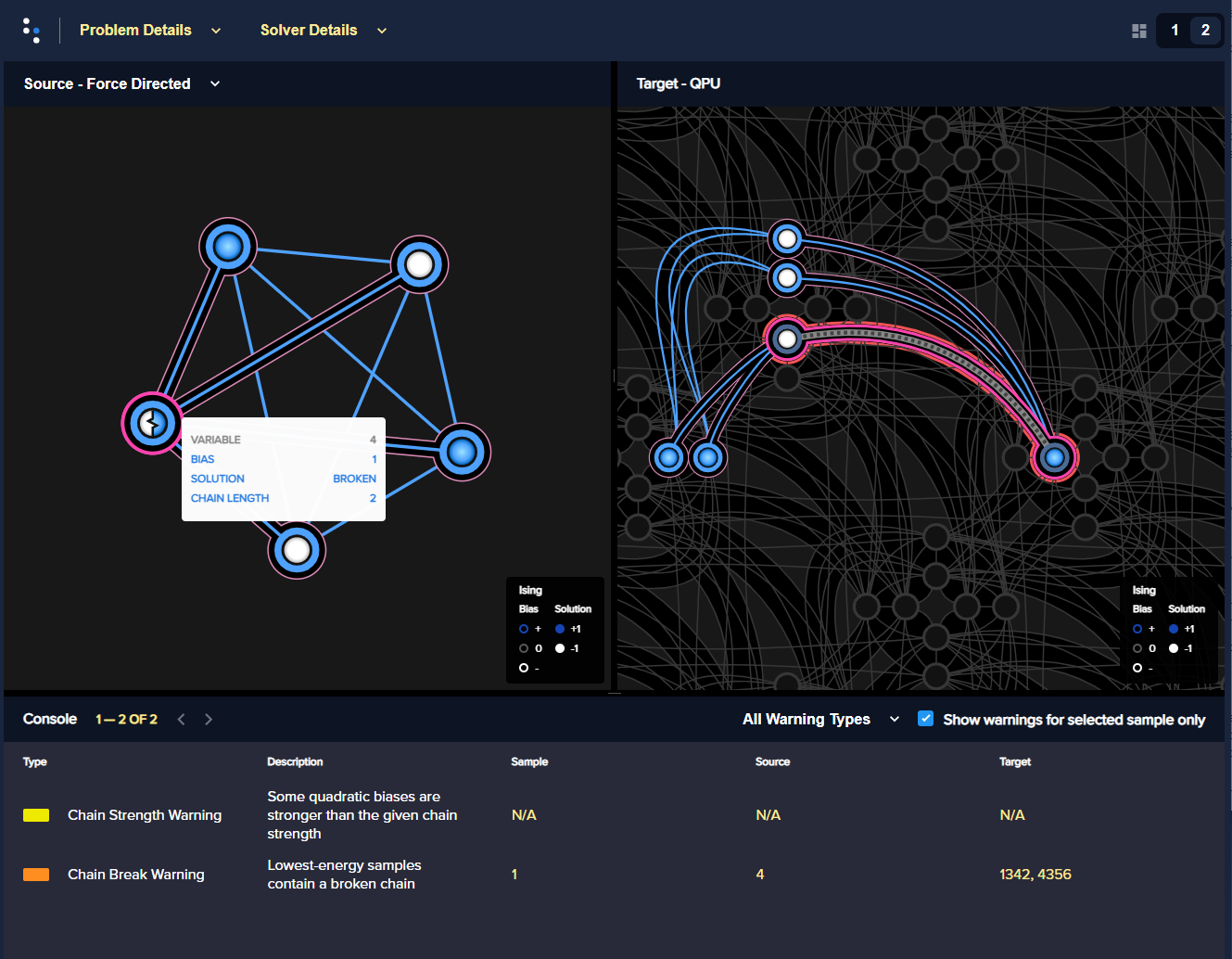
The logical problem, on the left, shows that the value for variable 4 is
based on a broken chain; the embedded problem, on the right, highlights the
broken chain (its two qubits have different values) in bold red.#